Data Processing

5 TersusMVP Mapper

5.1 Introduction

TersusMVP Mapper is a dedicated processing software for MVP S2. It automates the processing of raw data collected by the device to generate environmental point cloud data, panoramic images, trajectory, and more.

5.2 Recommended Computer Specifications

Operating System: Windows 11 64 bit

CPU: Core i9

RAM: 128GB

Storage: 1TB

5.3 Data Processing

5.3.1 Launch TersusMVP Mapper

The interface of TersusMVP Mapper is as follows.

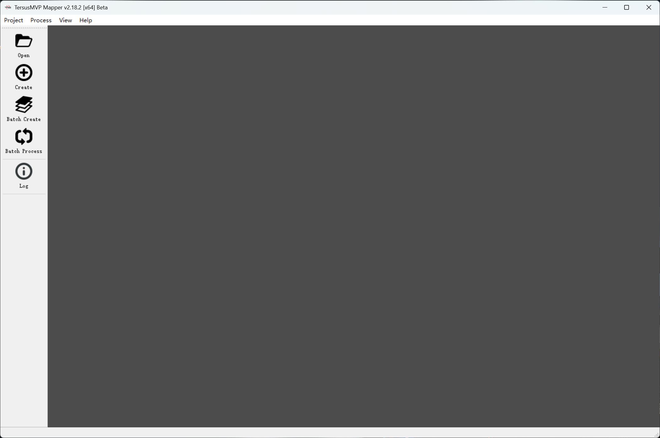Figure 5-1

5.3.2 Create project

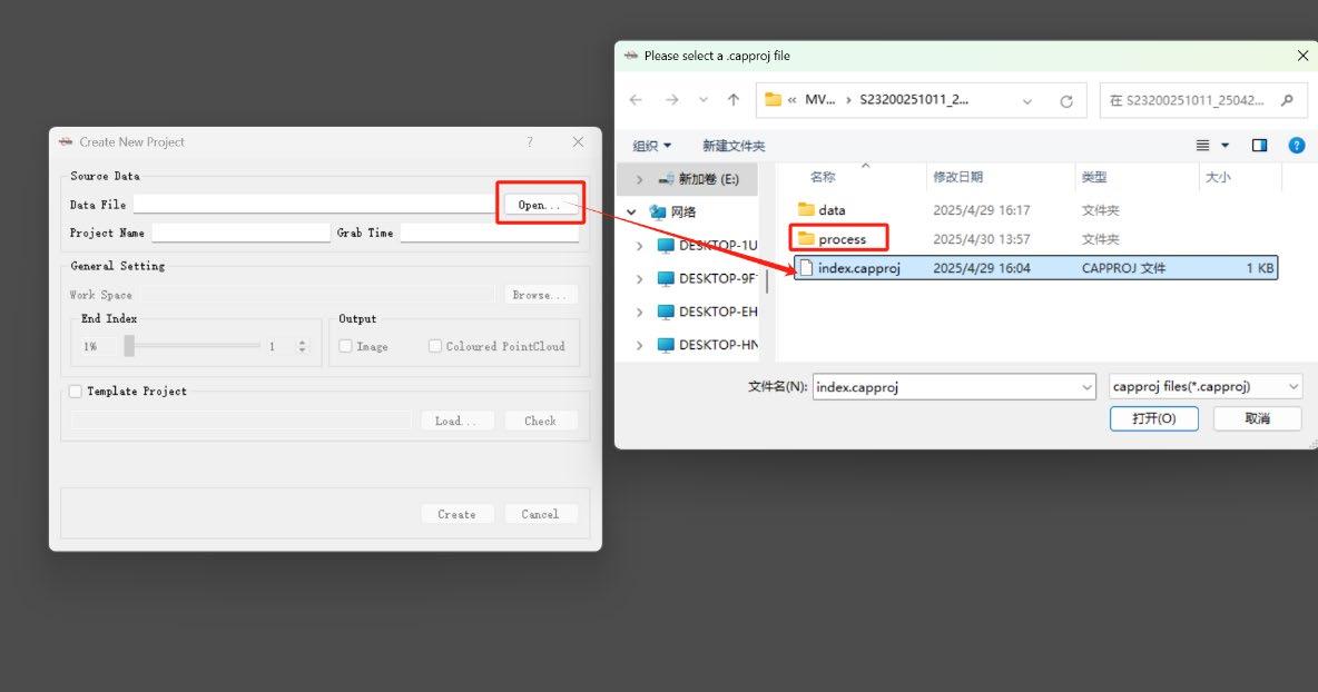
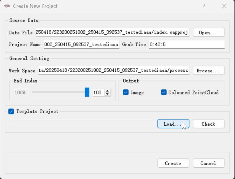
Click the "Create" button on the main interface to open the "Create New Project" dialog box.
Click the "Open" button to open “index.capproj” file and load the raw data.
Set the workspace and endpoint.
If image data is needed in the output, check the "Image" option; if colored point cloud data is needed, check the "Coloured PointCloud" option.
To use parameters from a template project, check "Template Project" and load the desired template.
Click the "Create" button to create the project, and the “process” folder will be generated in the project folder. Note: After creating a project, do not move the project workspace folder or modify its internal directory structure. Otherwise, errors may occur when reopening the project due to missing files.

Figure 5-2

5.3.3 Open Project

Click the “Open” button in the main software interface, and load “.procproj” file to reprocess a processed project with modified parameters.

5.3.4 Processing Configuration

Click

to change the processing configurations

Figure 5-3

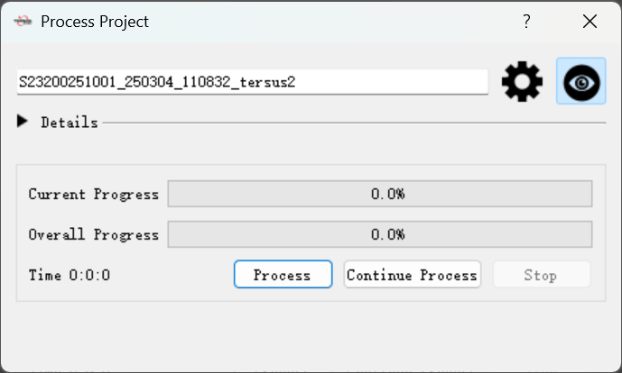
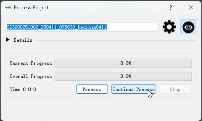
5.3.5 Start/Stop Processing

Click “Process” to start processing. Click "Stop" to cancel project processing. Note that canceling the processing may take some time.

5.3.6 Continue Process

After changing certain setting parameters, the user can use "Continue Processing" to reduce data processing time. Note: If a project has already been processed and you need to reset the output files or modify other configurations, please use the "Continue Processing" function.

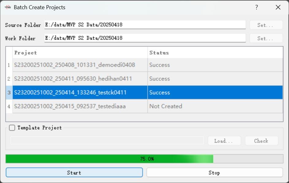
5.3.7 Batch Create

Set the data directory, which should contain the project folders copied from the device.
Set the working directory, where corresponding processing project folders will be automatically created based on the projects in the data directory.
If you need to use parameters from a template project, check the option and load the template project.
Click "Start" to generate the processing projects.

Figure 5-4

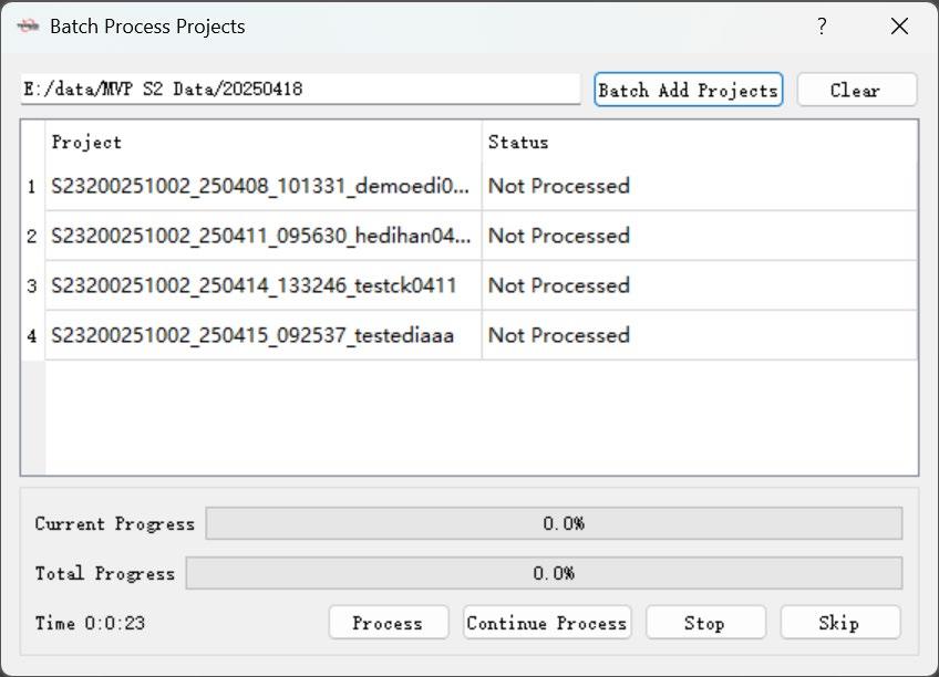
5.3.8 Batch Process

Batch add projects by selecting the folder that contains the processing projects.
Click "Process" to process all projects in sequence.
Click "Continue Processing" to continue processing each project in sequence.
Click "Terminate" to stop processing for all projects.
Click "Skip" to skip processing the current project.
Double-click a project in the project list to open the project configuration dialog and set parameters for that specific project.

Figure 5-5

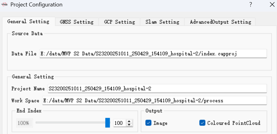
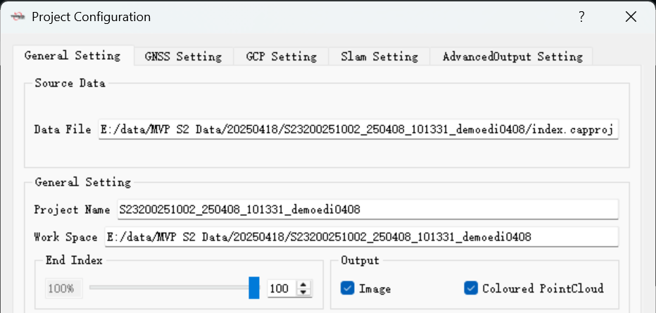
5.3.9 General Setting

In the general setting, you can set the endpoint and check the options for outputting images and colorized point cloud data. You can also set these parameters in the project creation process.

Figure 5-6

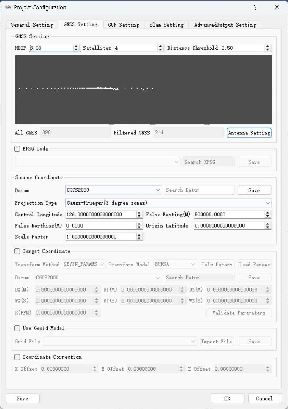
5.3.10 GNSS Setting

Figure 5-7

 HDOP: Horizontal Dilution of Precision, the smaller the value, the better the quality of the GNSS data. Set this parameter to adjust the GNSS data used in the calculation. It is typically set to 3.0.  Satellites: The number of satellites available for each GNSS data, the bigger the value, the better the quality of the GNSS data. It is typically set to 4.

 Distance Threshold: Represents the distance (in meters) at which an RTK data point is used. The default is 0.5 meters.  GNSS (white point): Represents the GNSS data points involved in the calculation. This can be used to view the distribution of GNSS points along the trajectory.  All GNSS: Represents all the GNSS data acquired.  Filtered: Represents the GNSS data used in the calculation. The number of GNSS data involved in the calculation can be changed by adjusting HDOP, the number of satellites, and the distance threshold. Note: Adjusting HDOP, the number of satellites, and the distance threshold will change the GNSS data involved in the calculation. It is generally fine to use the default parameters. During adjustments, be careful not to disrupt the even distribution of GNSS data.

5.3.11 Source Coordinate

The default coordinate system is CGCS2000, and the default projection is the Gauss-Krüger 3-degree zone projection. The central meridian, false easting, false northing, origin latitude, and scale factor need to be modified according to the actual situation. Note: Parameters such as Central Longitude must match those used in the actual project. Otherwise, calculation errors may occur.

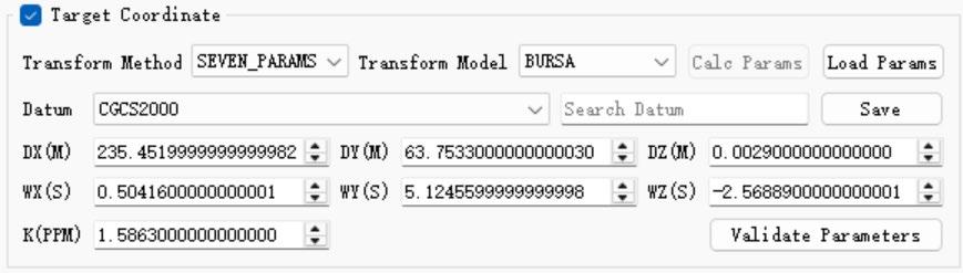
5.3.12 Target Coordinate

If coordinate transforming is required, make sure to check the Target Coordinate selection box. The software supports two types of coordinate transforming methods as follows. (1) If the user can provide the coordinate system and the corresponding Bursa seven parameters, enter the parameters in the designated fields. After clicking "OK," proceed with data processing according to the standard project workflow.

Figure 5-8

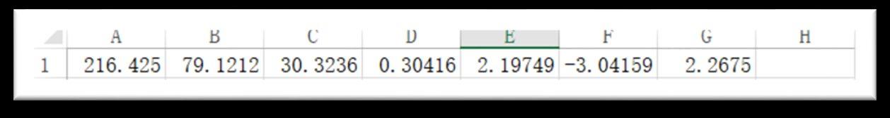
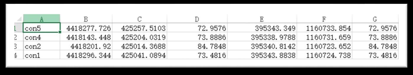
You can also click "Load Parameters" to import a CSV file containing the transformation parameters. The CSV file should follow the specified format (as shown in the figure), with values separated by commas by default.

Figure 5-9

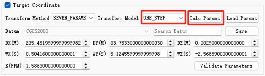
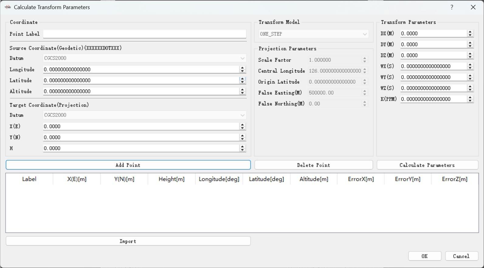
(2) If the user cannot provide the seven parameters, control points must be collected using a rover. A coordinate transformation file should then be created and imported into the software to calculate the seven parameters and complete the coordinate transformation. Select the transformation model ONE_STEP, then click the Calculate Parameters button.

Figure 5-10

The Calculate Transform Parameters interface will pop up. Then, click the Import button to import the coordinate transformation file.

Figure 5-11

The coordinate transformation file should use the following format: Point Name, Local Coordinate (North), Local Coordinate (East), Local Coordinate (Height),

Geodetic Latitude (B), Geodetic Longitude (L), Geodetic Height (H)

Figure 5-12

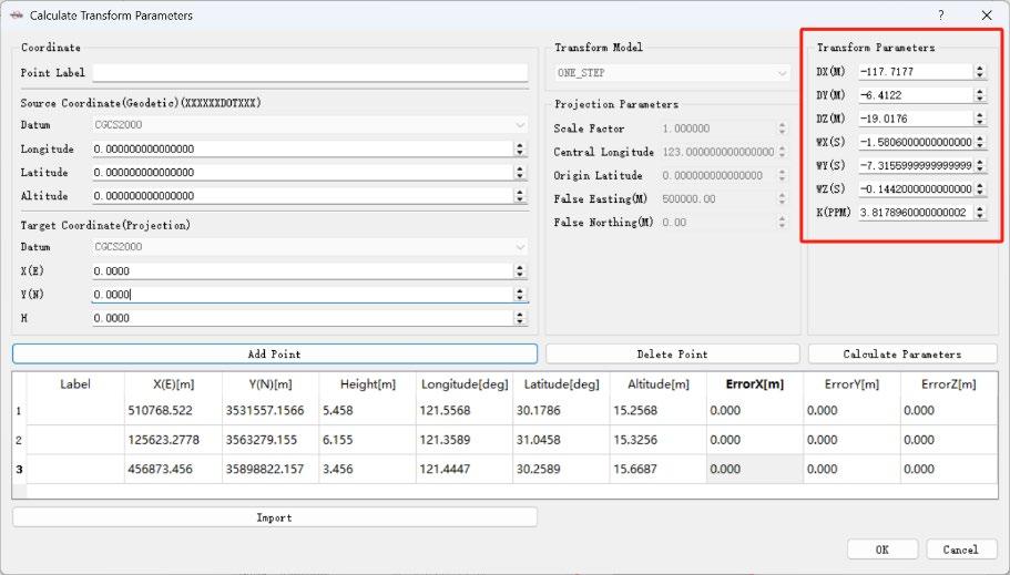
The latitude format should be XX degrees XX minutes XX.XXX seconds, and the longitude format should be XXX degrees XX minutes XX.XXX seconds. If the coordinate transformation is successful, the result will be displayed. After clicking "OK," proceed with data processing according to the standard workflow.

Figure 5-13

To verify the accuracy of the calculated seven parameters, follow these steps:

Enter the geodetic coordinates of the checkpoint into the left sidebar.
Click the Convert button.
Compare the output coordinates with the local coordinates of the checkpoint to assess the accuracy of the seven parameters.

Figure 5-14

Note: When calculating the seven parameters using this software, the transformation

model must be set to ONE_STEP, otherwise, a calculation error will occur.

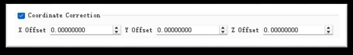
5.3.13 Coordinate Correction

The point cloud elevation calculated by the software is set to geodetic height by default. If the user needs to convert the geodetic height to another type of elevation, they can enter the corresponding parameters in the coordinate offset section and then perform the calculation.

Figure 5-15

5.3.14 GCP Setting

5.3.14.1 Import GCP

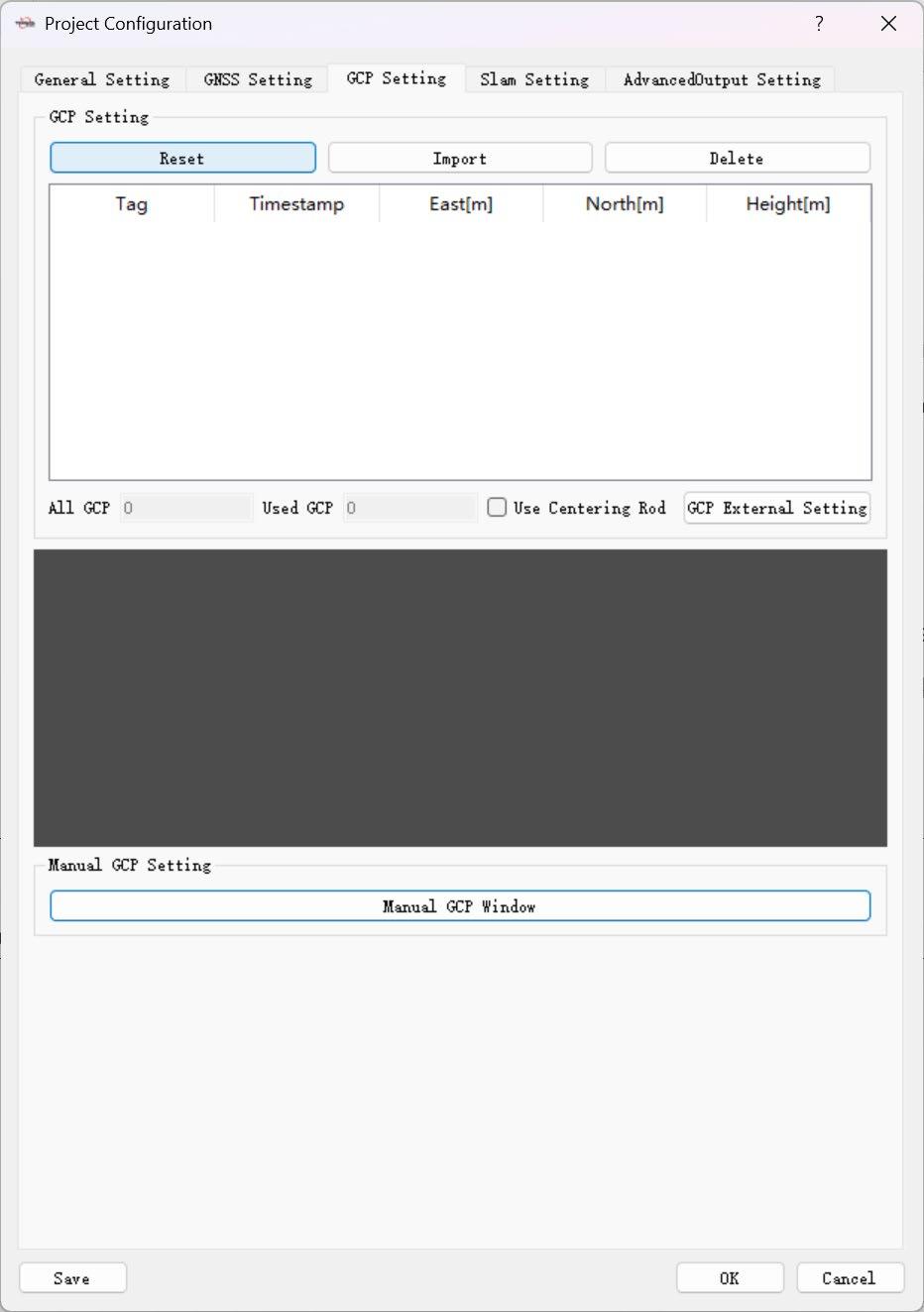
1．After creating a new project, if you need to import control points, click "GCP Settings", then click "Reset" to display the GCP list. The collection times of the points will be imported in sequence based on the order they were collected, labeled as "0, 1, 2, 3, 4, …".

Figure 5-16

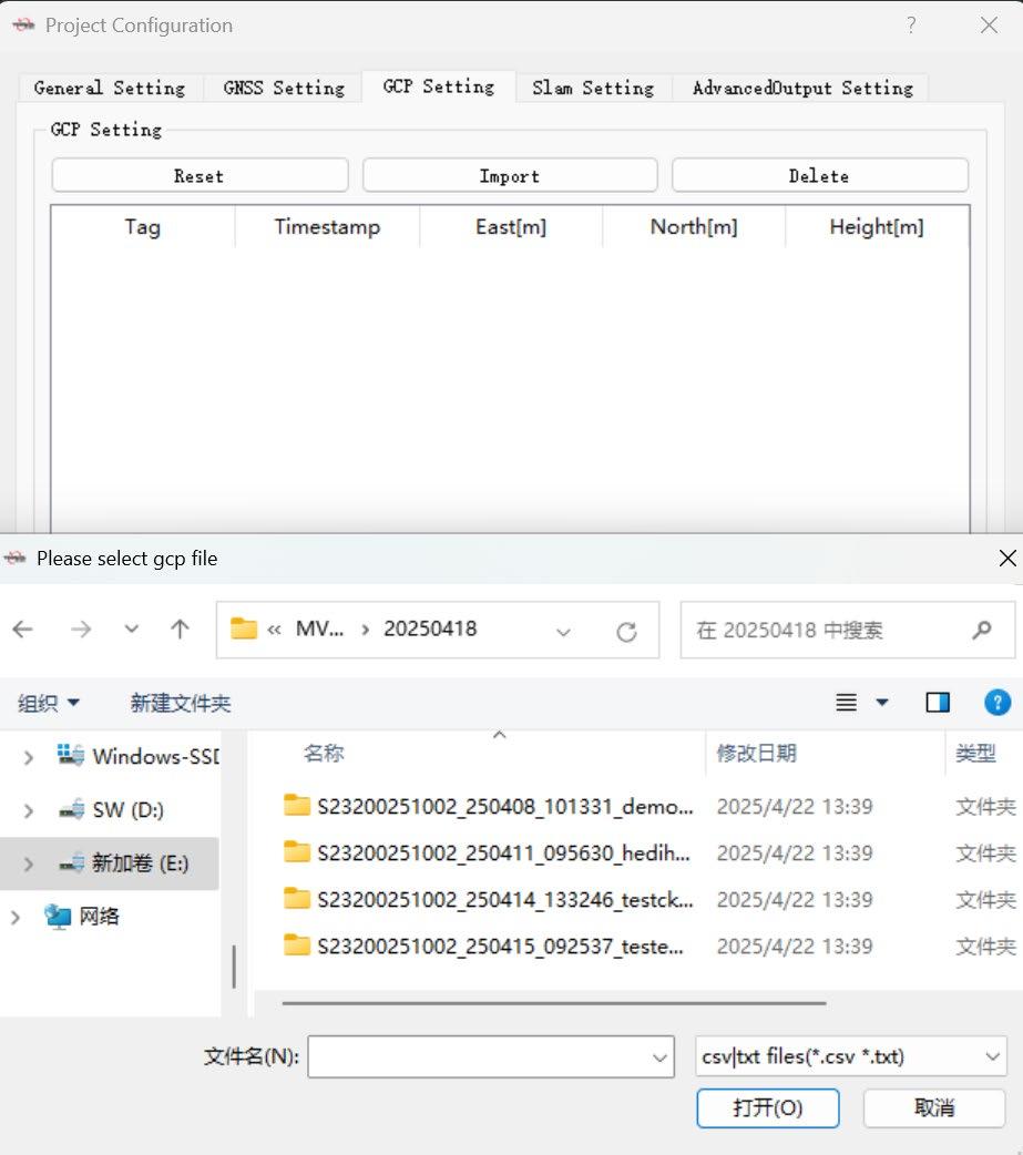
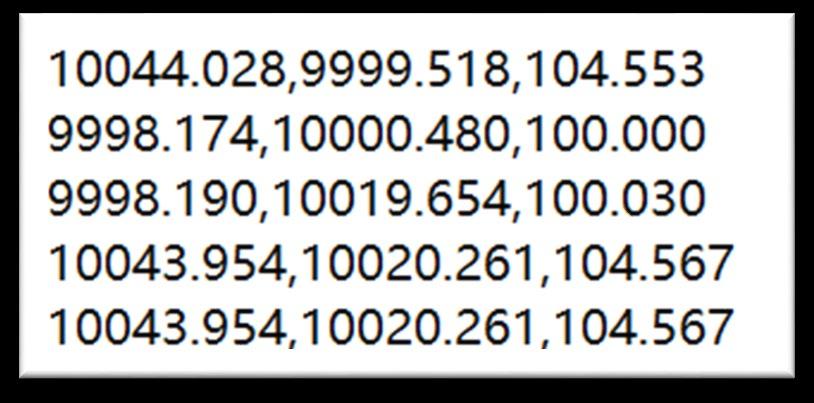
2．Store the control point coordinates in a TXT or CSV file, with each row containing the values in the order of East, North, Height, separated by commas. Click "Import " to load the coordinates based on the sequence in which the control points were collected. Finally, click "OK", then click "Process" to begin data calculation. Note: The order of the control points must exactly match the order in which the points were collected during the survey!

Figure 5-17

3．If the TXT or CSV file containing the control point coordinates uses separators other than commas between columns, or if the file includes malformed rows, irregular formatting, or non-numeric data such as Chinese characters, an error message will pop up. In this case, you need to carefully check the data and formatting of the control point file to ensure it meets the required structure.

Figure 5-18

4．For control point data already imported into the TersusMVP Mapper software, if a specific row is not needed, select that row and click "Delete " to remove it from the list. Note: The remaining number of control point entries must be no fewer than 4.

5.3.14.2 Manual GCP

1．Measure the coordinates of manual GCP in point cloud first, and then organize the target coordinates and the measured point cloud coordinates into the same table. Each row should include the point number, local coordinates (East X, North Y, Height Z), and point cloud coordinates (East X, North Y, Height Z) in that order. Finally, save the table in CSV format.

Figure 5-19

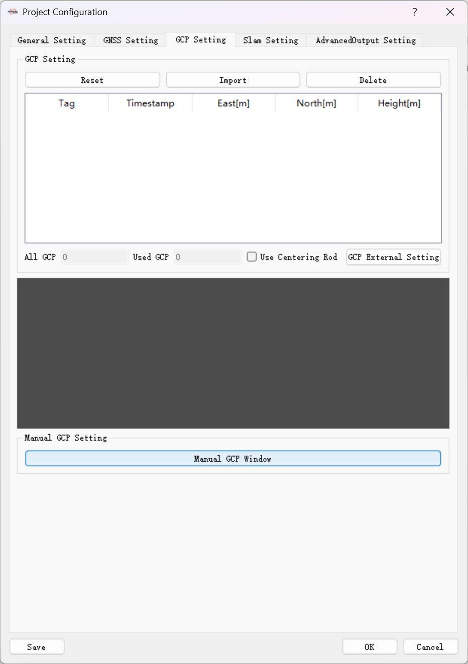
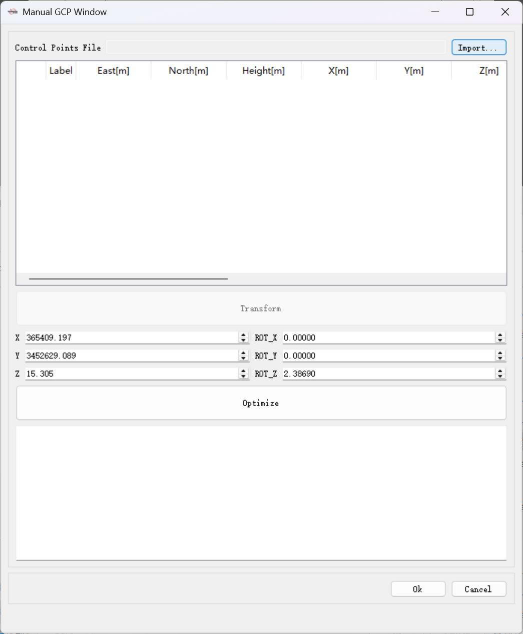
2．Click “Manual GCP Window” button, then click “Import” to import the CSV file.

Figure 5-20

3．At this stage, there are two cases: If the point cloud data is in relative coordinates, first click "Transform", then click "Optimize", followed by "Confirm", and finally "Continue Processing" to perform adjustment and coordinate transformation. If the point cloud data is in absolute coordinates, directly click "Optimize", then "Confirm", and finally "Continue Processing" to proceed with adjustment and coordinate

transformation.

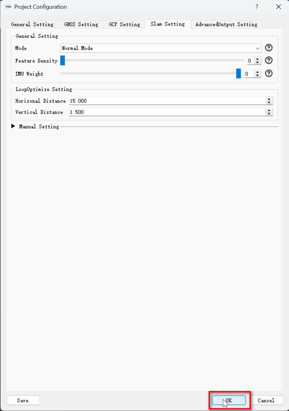
5.3.15 SLAM Setting

The parameters here usually do not need to be changed, the default settings are typically sufficient.

Figure 5-21

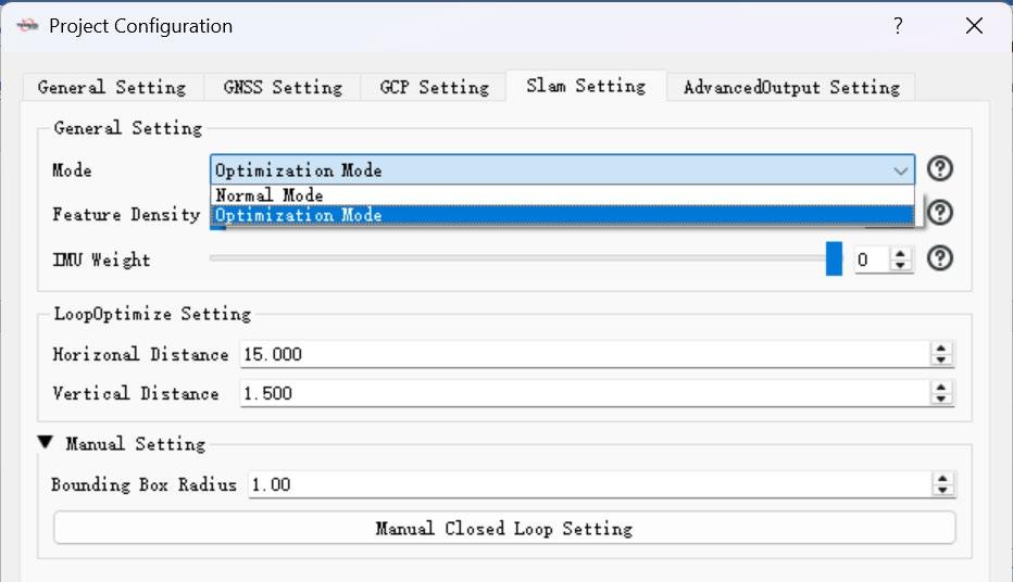
5.3.15.1 Slam Setting - General Setting

 Optimization Mode: When data cannot be properly processed due to a lack of features or weak textures, this function needs to be checked.  Feature Density: The number of features extracted from the environment. In conditions where features are scarce or the collection speed is fast, increasing the feature density can help prevent too few features from being used in the calculation, which could otherwise lead to processing failure.  IMU Weight: The confidence level of the IMU data during pose calculation. It generally does not need to be modified unless there are special circumstances. Note: Try using the optimization mode to solve weak-texture scenes first. If it still fails, then reduce the IMU confidence value and increase the feature point density value.

5.3.15.2 LoopOptimize Setting

 Vertical Distance: This is the vertical distance threshold for automatically searching loop closures. The default value usually does not need to be changed. However, if processing data from a multi-story environment with small inter-floor spacing (e.g., two floors close

together), it is recommended to reduce this value—typically setting it to 1.00 is appropriate.

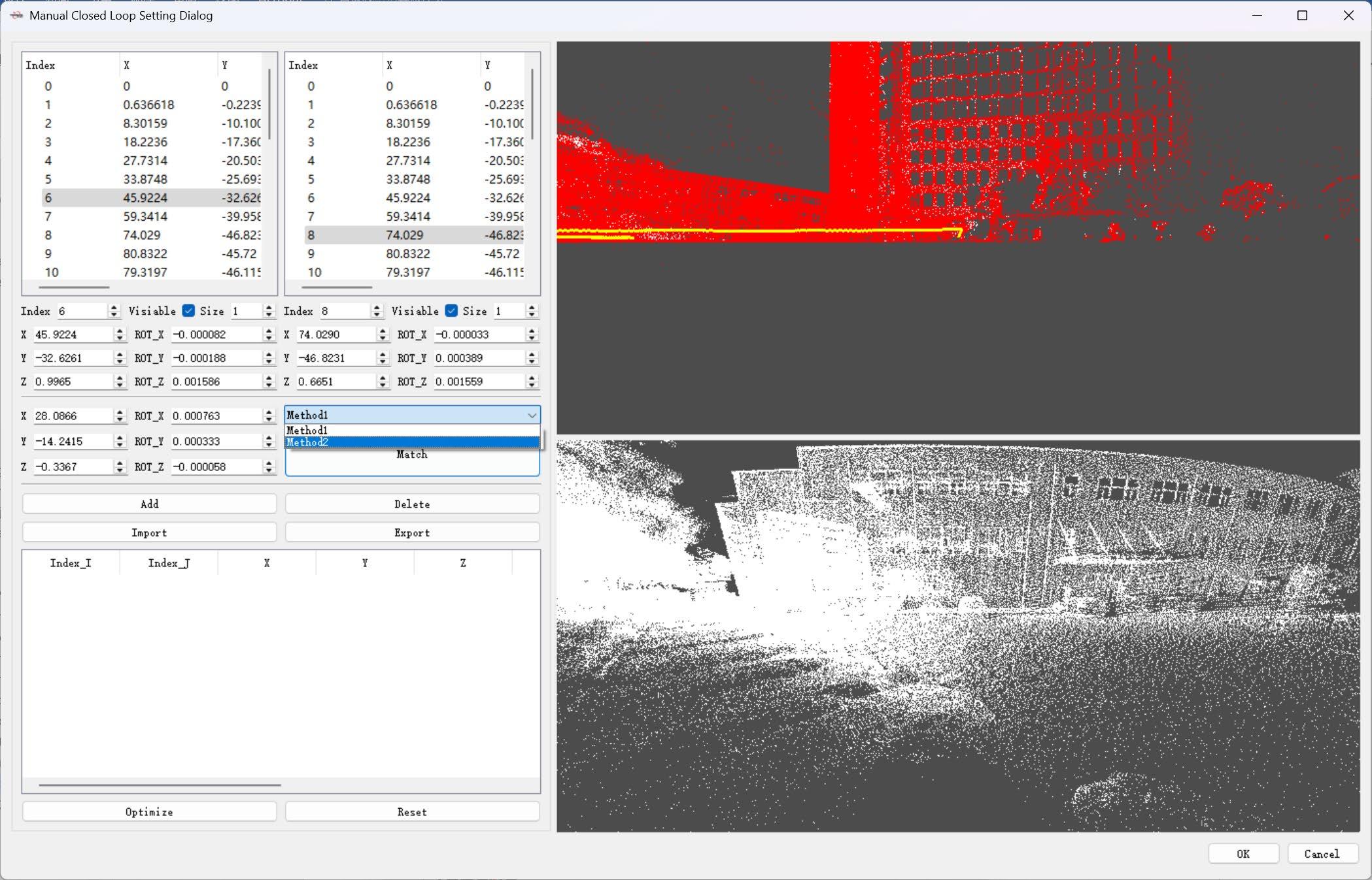
5.3.15.3 Manual Closed Loop Setting

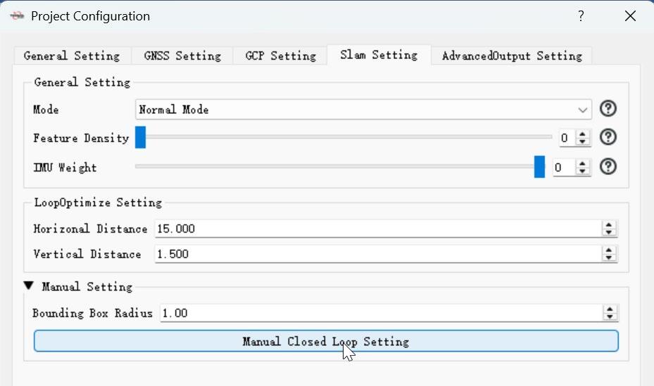
1．Open the project file that has already been processed, then go to Slam Setting> Manual Setting > Manual Loop Closure Setting.

Figure 5-22

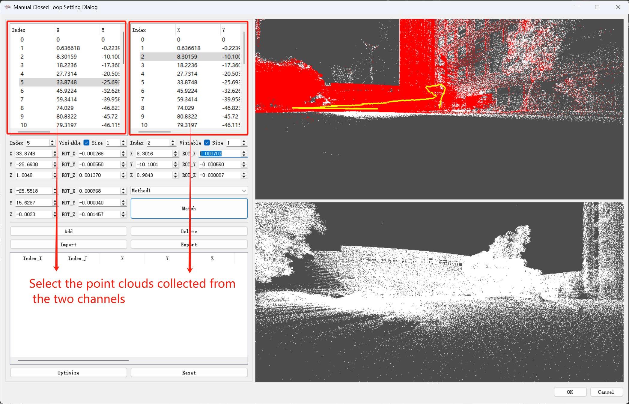
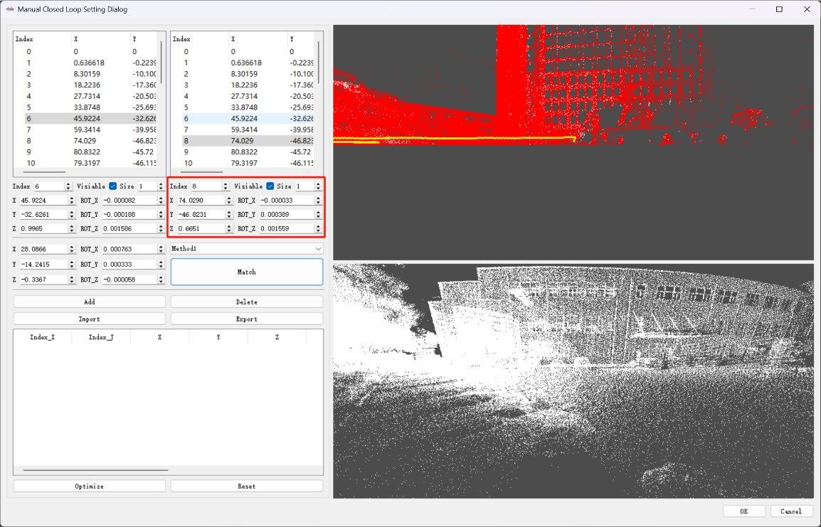
2．Select the point clouds collected from the two channels at the layering location, as shown in the figure.

Figure 5-23

3．Then click "Match". The bottom-right window will display the alignment result of the two layered point clouds. If the point clouds appear properly aligned without any visible layering, click "Add". After that, click "Optimize", and finally, click "OK".

Figure 5-24

4．Click “OK” to start processing the manually optimized results. (Note: If the data is fine after the first processing, there’s no need to reprocess it later. Do not move the file location, or the software may not be able to find the files for reprocessing.)

Figure 5-25

Click “Continue Process” to proceed with processing based on the manually closed loop optimized adjustments, as shown in Figure 5-26.

Figure 5-26

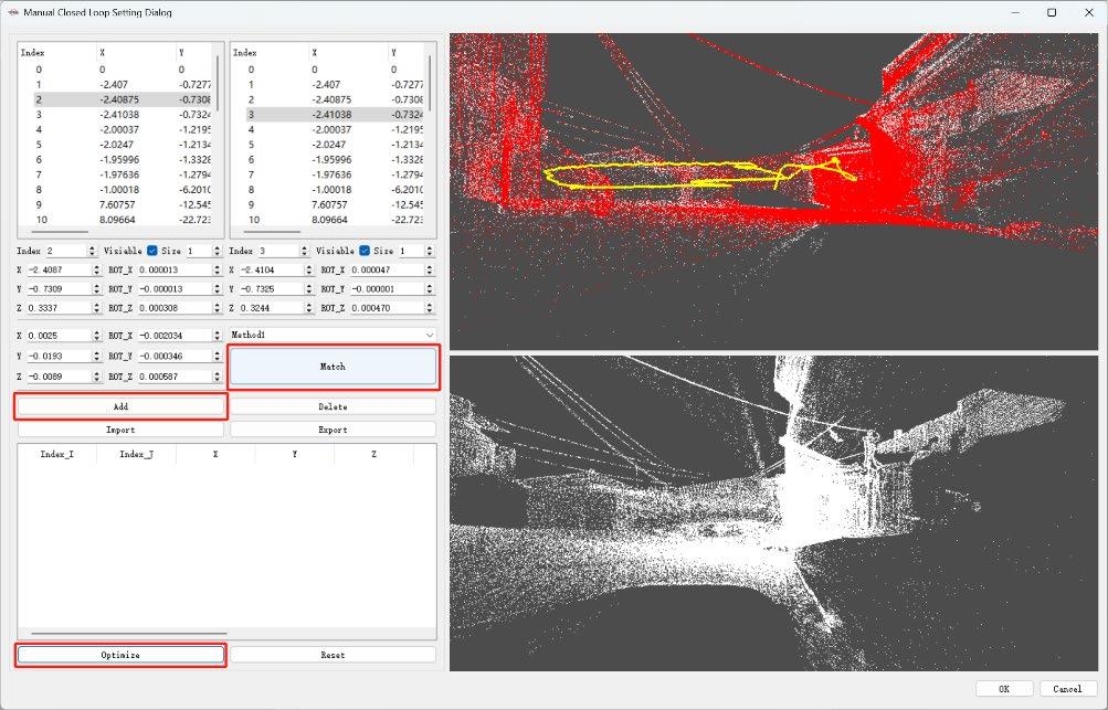
5．After matching, if the layered point clouds in the bottom-right corner still appear misaligned: (1) Adjust the values of X, Y, or Z (translation), or Rot_x, Rot_y, or Rot_z (rotation) in the lower right column. Then click “Match” again and observe the alignment of the two point cloud segments in the bottom-right corner. If they are no longer misaligned, click “Add”, then “Optimize”, and finally click “OK”, as shown in Figure 5-27.

Figure 5-27

(2) The manual loop closure is set to "Method 1" by default. If the stitching effect of "Method 1" is not good, you can switch to "Method 2" for "matching," as shown in Figure 5- 28.

Figure 5-28

"Import" and "Export": Users can export the manually closed point cloud data in CSV format. If other locations with layering are found in the processed point cloud, the CSV data of the first layered location should be "imported" and then used to stitch and match the point cloud

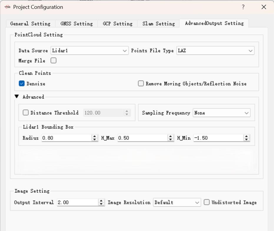
of the second layered location. Note: If the manually adjusted point cloud data from the first location with layering is not imported, the second location's point cloud may be successfully matched, but the first location's point cloud will still have layering issues. 5.3.16 AdvancedOutput Setting

Figure 5-29

5.3.16.1 PointCloud Setting

 Data Source: The data source for point cloud modeling in the S2 series is fixed to Lidar1 and cannot be changed.  Points File Type: Choose the output format for the point cloud data. Both LAS and LAZ formats are available, and they offer identical data quality. The LAZ format, however, requires less storage space.  Merge File: By default, TersusMVP Mapper software outputs point cloud data in 5- minute segments in LAS/LAZ format. If the user needs a single continuous LAS/LAZ file, they can enable the "Merge File" option.(For example, for 20 minutes of data, the default output would be 4 separate segments; if merging is enabled, the output will be one complete segment.)  Denoise: To remove noise from the point cloud.  Remove Moving Objects/Reflection Noise

 Remove Moving Objects/Reflection Noise: Remove moving objects from the point cloud, such as pedestrians, moving vehicles, and noise caused by reflections from glass surfaces or water bodies.

5.3.16.2 Advanced

 Remove Moving Objects/Reflection Noise  Distance Threshold: Small stratifications and noise points caused by long-range LiDAR scans can be removed. The larger the parameter setting, the more points will be deleted.  Lidar Bounding Box Radius: This refers to removing point cloud data within a cylindrical area centered around the LiDAR, with a default radius of 0.8 meters. H_Max: By default, point cloud data within 0.5 meters above the LiDAR is removed. H_Min: By default, point cloud data within 1.5 meters below the LiDAR is removed.

5.3.16.3 5.3.16.3 Image Setting

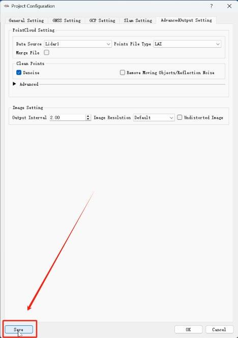
 Output Interval: The default value is 2, meaning one image is output for every two images.  Image Resolution: Adjust the resolution of the output panoramic image. 5.3.17 Template Project Users can save project parameters as a template. When creating a project or batch creating projects, loading the template project will automatically set the project parameters to those of the template, improving efficiency. Click the "Save Template" button in the dialog box to save.

Figure 5-30

6 TersusMVP Viewer

6.1 Introduction

TersusMVP Viewer is the companion visualization software for the MVP S2. It enables the display of processed results from the Mapper software, supports ultra-fast loading of massive point cloud datasets, and allows real-world imagery to be overlaid and synchronized with point cloud data. The software also supports real-world measurements, point cloud clipping, and various display modes including color, intensity, and elevation views.

6.2 Recommended Computer Specifications

Operating System: Windows 11 64 bit

CPU: Core i7

RAM: 32GB

Storage: 1TB

6.2.1 Launch TersusMVP Viewer

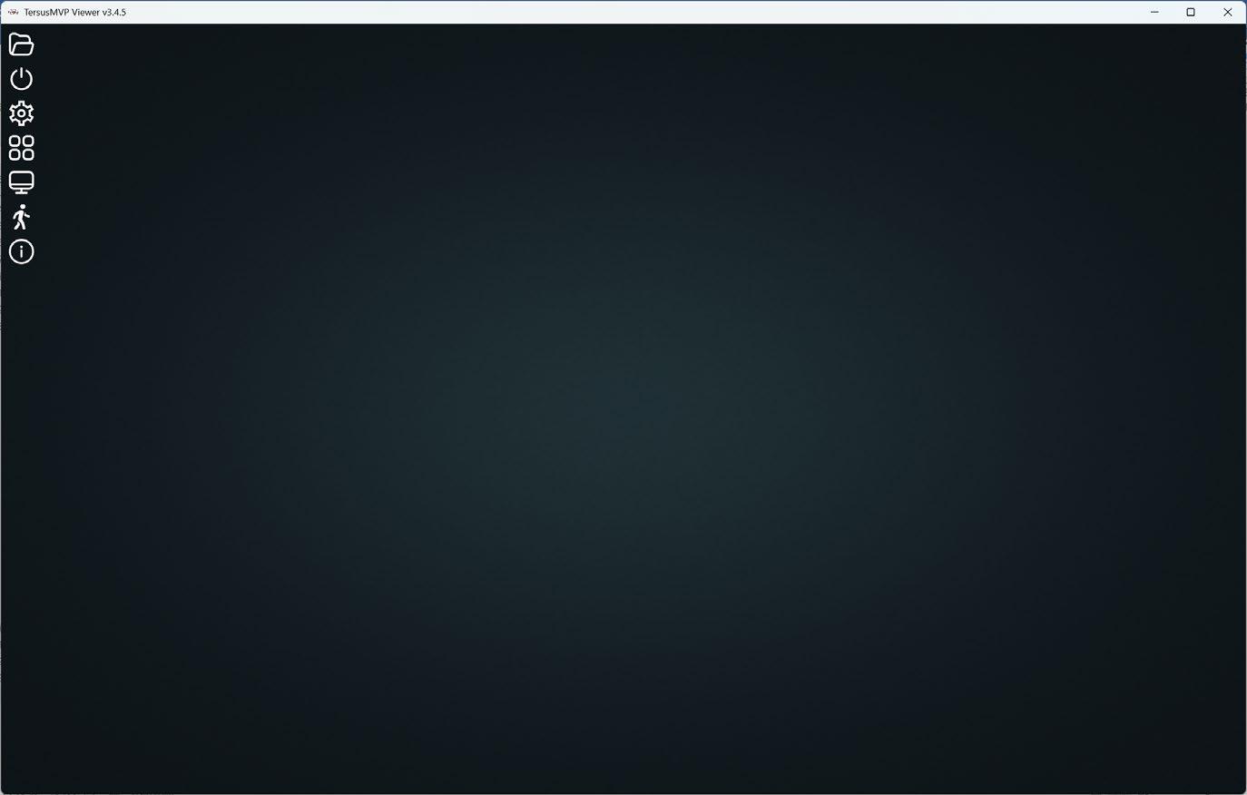
The interface of TersusMVP Viewer is as follow.

Figure 6-1

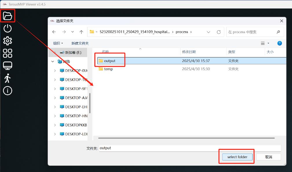
6.2.2 Open Point Cloud Data

Click the "Open Point Cloud" button on the main interface and select the “Process\output” folder.

Figure 6-2

Note:

Do not select any folder other than the output folder, otherwise an error message will appear indicating the folder selection is incorrect.
If you've already loaded the data into the Viewer software and need to update the .las/.laz point cloud files in the output folder, please delete the automatically generated “tiles_data” folder inside the output directory first.
The point cloud file names in the output folder must contain the word "points", such as “xxxx points xxxx.las”.

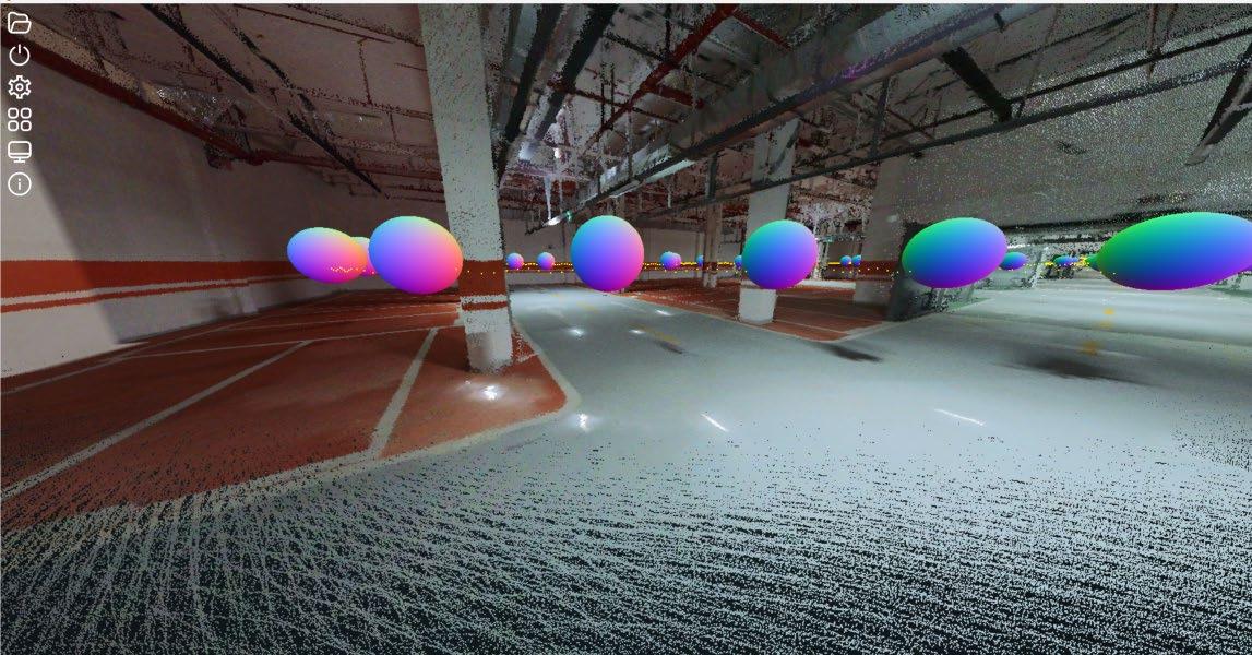
6.2.3 Overlay Panoramic Images with Point Cloud Data

Left-click to pan, right-click to rotate, and scroll the mouse wheel to zoom in and out.
Double left-click on the panoramic sphere to view the panoramic image at the current location.
Right-click to exit the panoramic sphere.
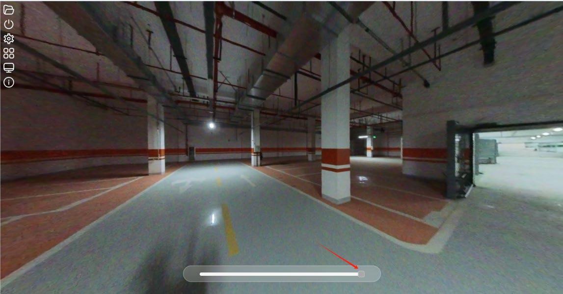
Drag the gray square block to adjust the transparency of the panoramic image, enabling overlay display with the point cloud data.

Figure 6-3

Figure 6-4

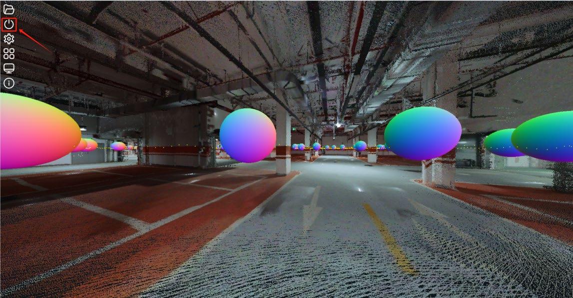
6.2.4 Reset Point Cloud

Click the "Reset Point Cloud" button to clear the current data.

Figure 6-5

Figure 6-6

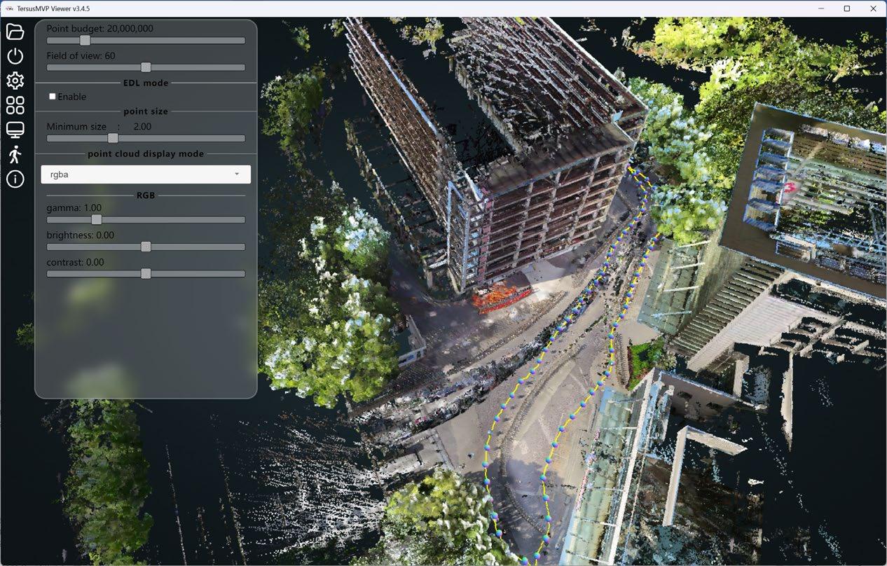
6.2.5 Set The Point Cloud Display Mode.

The point cloud display mode can be set to: intensity, colored intensity, classification, rgba, elevation. Gamma: Also known as the grayscale coefficient, it is used to adjust the ratio of brightness and contrast. Increasing the gamma value enhances the grayscale contrast, while decreasing it reduces the contrast. In most cases, the default gamma value works well and does not require adjustment. Brightness: Adjusts the overall lightness or darkness of the point cloud display. Contrast: Modifies the difference between the light and dark areas in the display to enhance visual clarity.

Figure 6-7

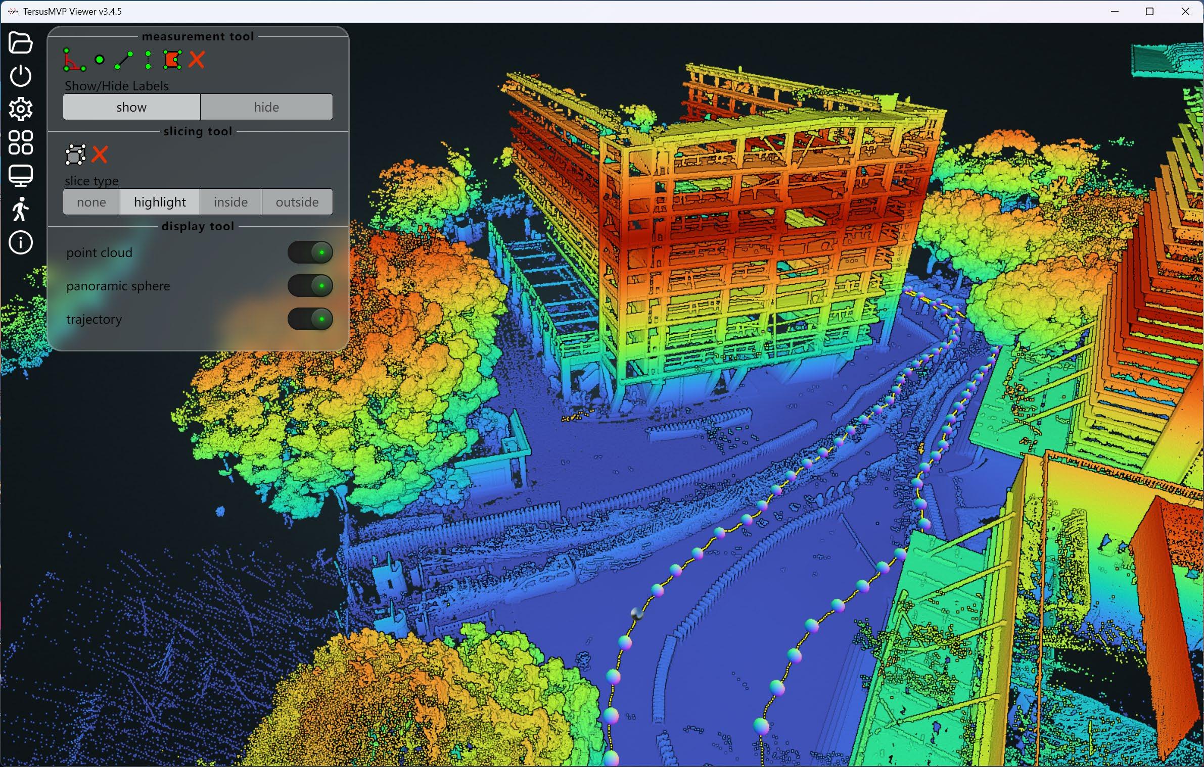
6.2.6 Point Cloud Tools

The point cloud tools include: measurement tool, slicing tool, display tool.

Figure 6-8

6.2.6.1 Measurement Tool

Measurement tool include: Angle measurement, Point measurement, Distance

measurement, Height measurement, Area measurement.

Click

to clear any measurement results. Click “Hide” to hide measurement values.

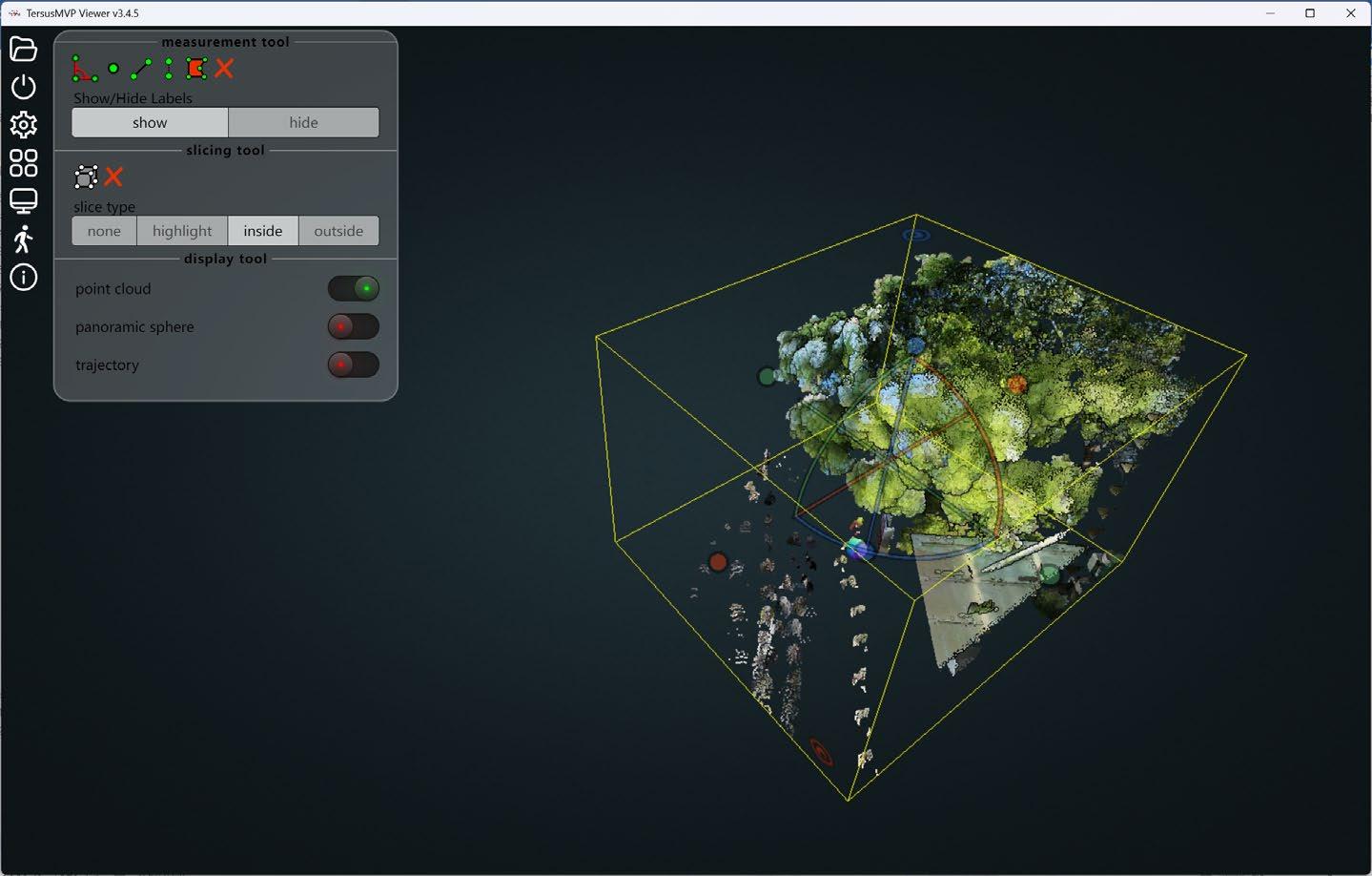
6.2.6.2 Slicing tool

Left-click with the mouse to activate the clipping bounding box. Adjust the size of the bounding box by dragging the colored spheres in each direction. Inside: show the point cloud inside the clipping bounding box.

Figure 6-9

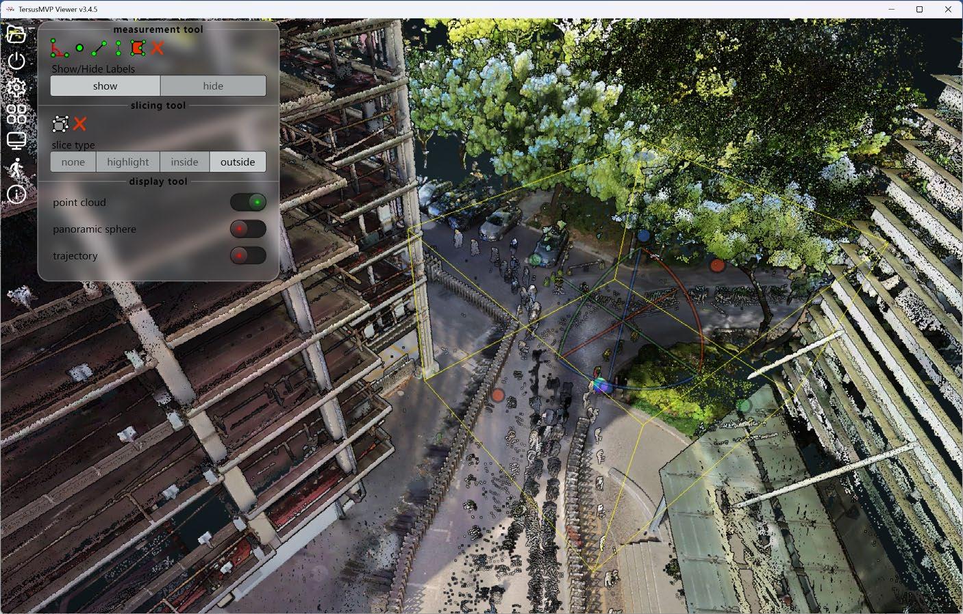
Outside: show the point cloud outside the clipping bounding box.

Figure 6-10

❌: Cancel clipping

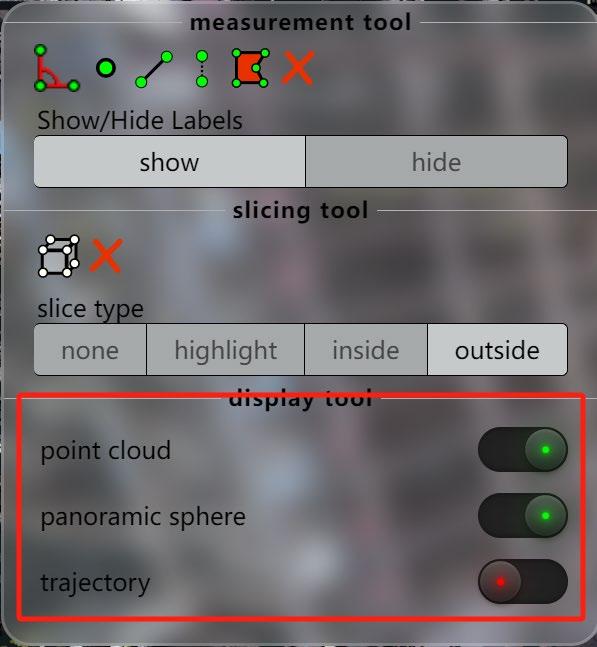
6.2.6.3 Display tool

Control whether to display the point cloud, panoramic spheres, and trajectory.

Figure 6-11

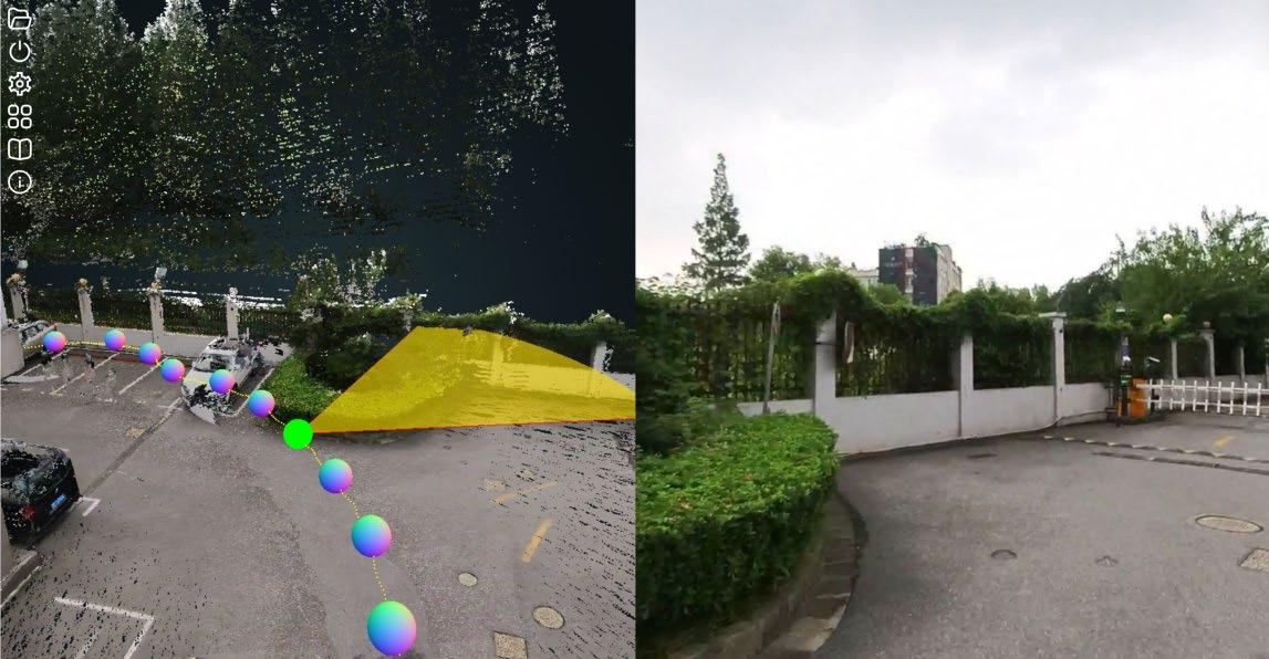
6.2.7 Split-screen Display of Panoramic Images and Point Cloud.

Click

, then click the panoramic sphere with the left mouse button to view the corresponding real-world image on the right side. The current field of view (highlighted in yellow) will be displayed on the left side.

Figure 6-12