Tools

• Area Perimeter

• Azimuth Distance

• Offset Point

• Rotation Point

• Two Points Intersection

• Four Points Intersection

• Intersection Angle

• Earthwork

• Angular Bisector

• Grid to Ground

• Line Segmentation

• Points Avg

• Parameters

• Area Division

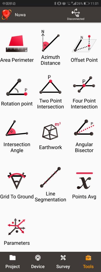
Figure 5.1[]{#_Toc6831 .anchor} Functions under Tools

Area Perimeter

This tool is used to calculate area and perimeter. The points can be imported from the point library by clicking the list icon on the upper right corner. The unit is meter for perimeter and square meter for area.

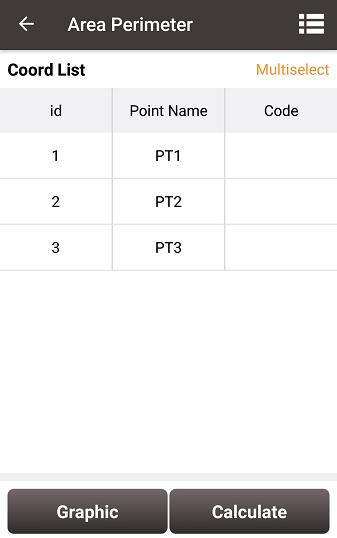
Figure 5.2[]{#_Toc14013 .anchor} Area Perimeter interface

[Graphic]: shows the closed polygon formed by the points.

[Calculate]: calculates the area and perimeter of the closed polygon.

[Multiselect]: enters point edit interface to inverse or delete.

Note: The calculation results are all plane results (point elevation does not participate in the calculation). It is suitable for all sections in this chapter except section 5.3 Offset Point.

Azimuth Distance

There are two kinds of azimuth distance calculation: point to point, and point to line. The points can be imported from the point library.

5.2.1 Point to Point Distance

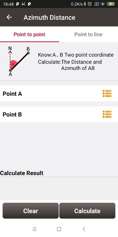
Figure 5.3[]{#_Toc22767 .anchor} Azimuth Distance -- Point to Point

Import point A and point B from the point library.

[Calculate]: calculate the distance between the two points and the azimuth.

[Clear]: clear the result.

5.2.2 Point to Line Distance

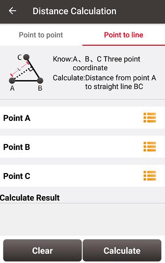
Figure 5.4[]{#_Toc14014 .anchor} Azimuth Distance -- Point to Line

Import points from the library to calculate the distance from point A to line BC.

[Calculate]: calculate the distance.

[Clear]: clear the result.

Offset Point

5.3.1 Offset point

Given the azimuth of point A & P, AP's horizontal length L and height H, calculate the coordinate of P. The steps are as follows:

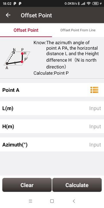
Figure 5.5[]{#_Toc2018 .anchor} Offset Point interface

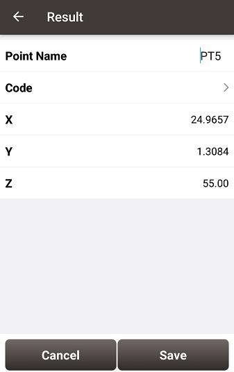
Figure 5.6[]{#_Toc27780 .anchor} Offset Point calculation result

[Calculate]: calculate the coordinate of point P.

[Clear]: clear the current result.

5.3.2 Offset point from line

Given the coordinates of point A and B, the distance L from B to C or from A to C, the offset D from AB line and the height difference H, calculate the coordinate of point P.

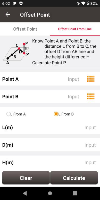
Figure 5.7[]{#_Toc9675 .anchor} Offset point from line

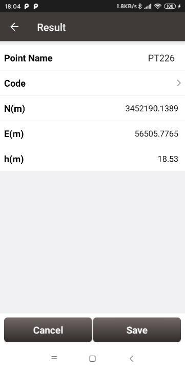
Figure 5.8[]{#_Toc15356 .anchor} Offset point from line calculation result

[Calculate]: calculate the coordinate of point P.

[Clear]: clear the current result.

Rotation Point

Given the coordinates of point A, B and the rotation angle (clockwise), calculate the coordinate of point B after rotation.

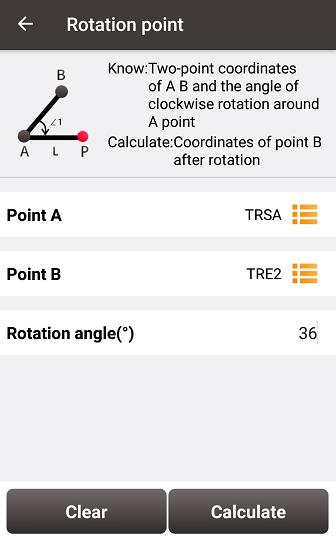
Figure 5.9[]{#_Toc18064 .anchor} Rotation Point interface

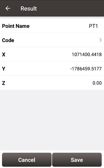
Figure 5.10[]{#_Toc28128 .anchor} Rotation Point Calculation result

[Calculate]: calculate the coordinate of point B after rotation.

[Clear]: clear the result.

Two Points Intersection

There are two types of models listed below:

• Model 1: Given the coordinates of point A and B, the angle α between line AB and AP, the angle β between line AB and PB, calculate the coordinate of point P.

• Model 2: Given the coordinates of point A and B, the length of line AP and BP, calculate the coordinate of point P.

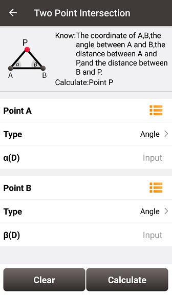
Figure 5.11[]{#_Toc15200 .anchor} Two Point Intersection -- Angle

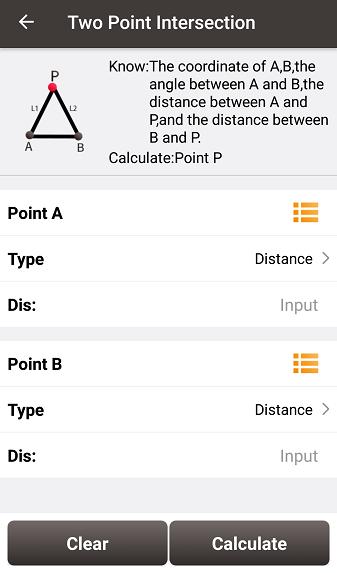
Figure 5.12[]{#_Toc13437 .anchor} Two Point Intersection -- Distance

[Calculate]: calculate the coordinate of the intersection P on both sides, left, or right.

[Clear]: clear the result.

Four Points Intersection

Given the coordinates of point A, B, C and D, calculate the coordinate of the intersection point P between line AB and line CD.

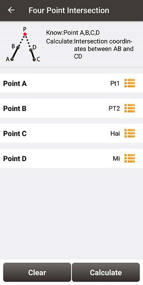
Figure 5.13[]{#_Toc23960 .anchor} Four Point Intersection interface

Figure 5.14[]{#_Toc28089 .anchor} Four Point Intersection result

[Calculate]: calculate the coordinate of the intersection P.

[Clear]: clear the result.

Intersection Angle

Given the coordinates of point A, B and C, calculate the angle ∠ABC

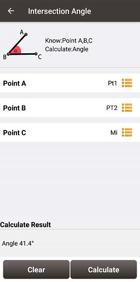
Figure 5.15[]{#_Toc232 .anchor} Intersection Angle calculation

[Calculate]: calculate the angle ∠ABC.

[Clear]: clear the result.

Earthwork

The detailed earthwork process is as below.

(1) Select all surface points to be calculated for earthwork from the point library, and add them to the list of All Points.

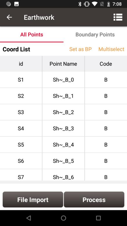
Figure 5.16[]{#_Toc18004 .anchor} Select all surface points to be calculated

(2) Select the boundary points from the list of All Points, and set them as BP to add them to the list of Boundary Points. Sort the boundary points in order by moving up and down.

![Screenshot_20210927-070904](/img/geosystems/field-controllers/nuwa/media/image391.jpg)

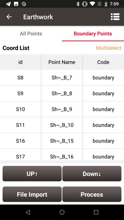
Figure 5.17[]{#_Toc20658 .anchor} Select the boundary points

(3) Click [Process], the software will first ask the path to save the surface file to be generated.

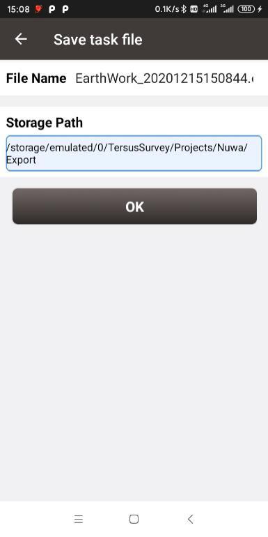
Figure 5.18[]{#_Toc8814 .anchor} File name and storage path for the earthwork

(4) The software will generate a triangulation network from the selected surface points through specific rules.

(5) Input the reference height, the software will calculate the volume formed between each triangulation network and the reference height, and calculate the fill and excavation amount in total.

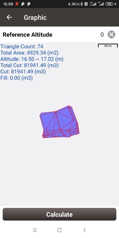
Figure 5.19[]{#_Toc7346 .anchor} Earthwork calculation result

Angular Bisector

Given the coordinates of point A, B and C, and the length of BP in which P is a point on the angular bisector of the angle ∠ABC, calculate the coordinate of point P.

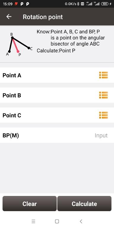
Figure 5.20[]{#_Toc28490 .anchor} Intersection Angle calculation

[Calculate]: calculate the coordinate of point P.

[Clear]: clear the result.

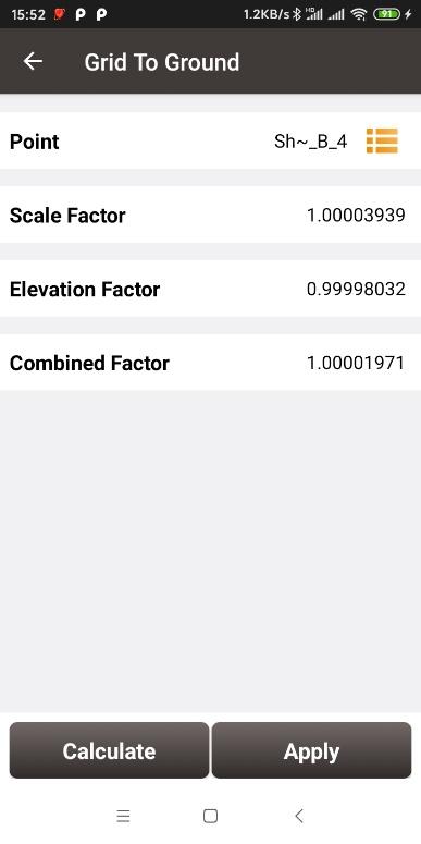
Grid to Ground

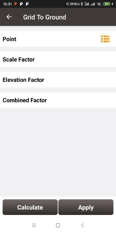
Since the GNSS measurement gets the plane grid coordinates by projection, there are deformation caused by the projection and the deformation caused by the curvature of the earth. If the length between points A and B measured by GNSS receiver will be different from the length between points A and B measured by optical instruments such as total station, so when the measurement area is large, it is necessary to consider this tool to realize the correction of grid coordinates to ground coordinates.

By selecting a point as the datum and clicking Calculate, the software will calculate the correction factor based on the location of the datum, and then click Apply to apply the correction factor to the project. If you find that the software calculates the scale factor incorrectly, or if you learn the correct scale factor in some other form, you can modify it manually.

+----------------------------------------------------------------------------------------------------------------------------------------------+----------------------------------------------------------------------------------------------------------------------------------------------+ | | | | | | | Figure 5.21[]{#_Toc22756 .anchor} Grid to Ground interface | Figure 5.22[]{#_Toc16977 .anchor} Calculate the correction factors | +----------------------------------------------------------------------------------------------------------------------------------------------+----------------------------------------------------------------------------------------------------------------------------------------------+

After clicking Apply, return to the point library to see, the point details of the measured points in the point library add the display of ground N, E and h coordinates, and the distance between these points and the datum under the ground coordinates are worth to reformat.

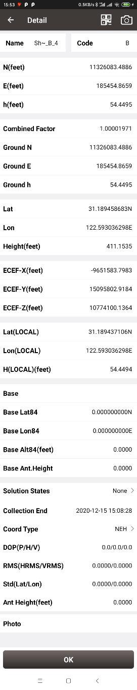
Figure 5.23[]{#_Toc23609 .anchor} Point detail after applying the calculation

Line Segmentation

Given AB line, calculate the equivalent points or equidistant points on line AB.

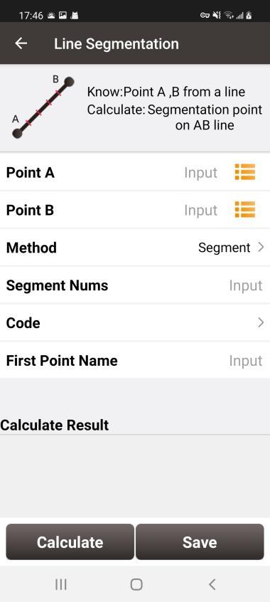
Figure 5.24[]{#_Toc2808 .anchor} Line Segmentation

[Segment method]:By number of segments or by interval length

[Code]: Calculation points code

[First Point Name]: Calculation points name and naming rule

[Calculate]: Calculate points

[Save]: Save the calculation points to the point library

Points Avg

This tool is used to calculate the average points. Points can be imported from the point library by clicking the list icon on the upper right corner or by clicking the Add button. Click the Calculate button to calculate the average result for all selected points and display the difference between the selected points and the average result.

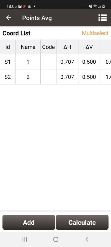
Figure 5.25[]{#_Toc19500 .anchor} Points Avg

Parameters

Seven Parameter and Three Parameter methods are introduced in this section.

Seven Parameter: this method can cover long distance range, generally more than 50 km. At least three known points are required in local datum and in WGS84 system before calculating.

Three Parameter: at least one known point is required. This method can cover short distance range; the accuracy is determined by working area and decreased with the distance.

The following is an example of Seven Parameter. Click [Project] -> [Parameters] to enter the following interface.

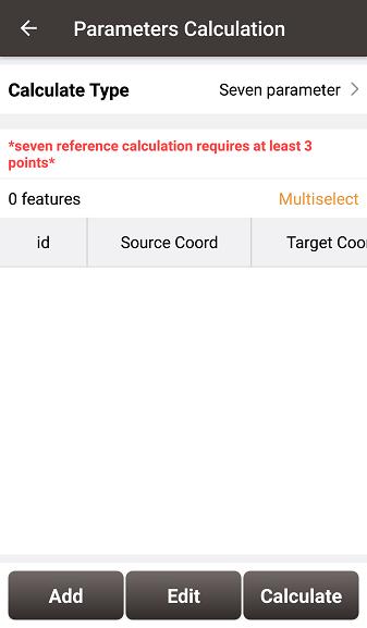
Figure 5.26[]{#_Toc3037 .anchor} Parameters Calculation

Select seven parameter for Calculate Type, click [Add] on the bottom left to input the known points.

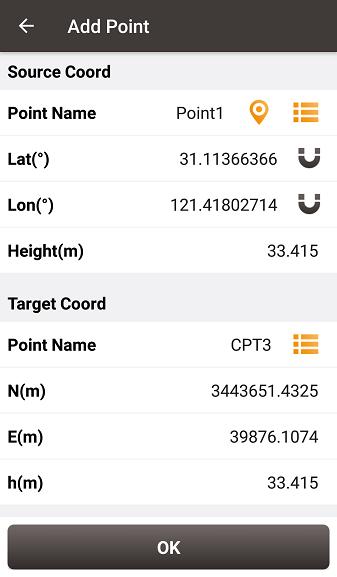
Figure 5.27[]{#_Toc32151 .anchor} Add Point for calculation

For the Source Coordinate, input Latitude, Longitude and Height by manual input, collected from a Tersus receiver or selected from the survey point list. For the Target Coordinate, input the local values from manual input or selected from the control point list.

• Manual input

Input the point position according to the format required. The latitude/longitude format can be changed by clicking the icon on the right.

• Point library

Click [] to load points from point library. Points can be added by clicking [Add] in the Point interface.

• Smooth Acquisition

Click [] to start smooth acquisition through Tersus receiver.

After points are added, click [Calculate] on the bottom right to do the parameter transformation. The result is shown as below screenshot:

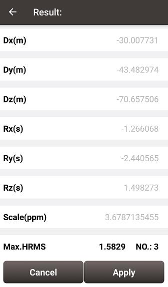
Figure 5.28[]{#_Toc12813 .anchor} Parameters Calculation Result interface

Note: Before this calculation, please make sure that the project parameters (ellipsoid, projection, etc.) are used correctly.

After the calculation is completed, click [Apply] to apply to the datum transformation parameters of the current project coordinate. When Max.HRMS is too large, the software will prompt a notice of whether continue to apply if the value is too large; if you click [Cancel], it will not be applied to the datum transformation parameters.

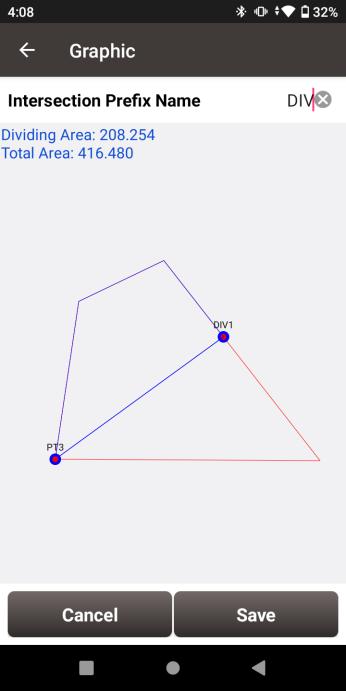
Area Division

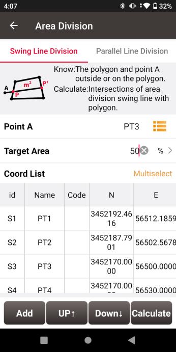
There are two methods of area division: swing line division and parallel line division.

Swing Line Division refers to calculating a straight line passing through point A on or outside the polygon, dividing the polygon so that the left part of the line is the target area, and calculating the intersection points of the line and the polygon.

Parallel Line Division refers to calculating a line parallel to the line between point A and point B, dividing the polygon so that the left part of the line is the target are, and calculating the intersection points of the line and the polygon.

+-----------------------------------------------------------------------------------------------------------------------------------------------------------------------+-----------------------------------------------------------------------------------------------------------------------------------------------------------------------+ | | | | | | | Figure 5.29[]{#_Toc9990 .anchor} Area Division Parameters | Figure 5.30[]{#_Toc2956 .anchor} Area Division Results | +-----------------------------------------------------------------------------------------------------------------------------------------------------------------------+-----------------------------------------------------------------------------------------------------------------------------------------------------------------------+

Select Swing Line Division or Parallel Line Division, select the point A of the swing line or the point A and point B of the parallel line, enter the target area as a percentage or a fixed value, select points to form the polygon in order in the list, then click Calculate. The software will calculate and draw the division line. Check and input the prefix of the intersection points to save them to the point database.