Survey
-
Survey
-
Point Stakeout
-
Line Stakeout
-
Static Survey
-
Site Calibration
-
Survey Config
-
Base Shift
-
Road Stakeout
-
Surface Stakeout
-
CAD Stakeout
-
CAD Survey
-
Visual Positioning
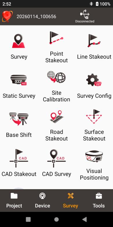
Figure 4.1[]{#_Toc2278 .anchor} Functions under Survey
Survey
The Survey interface includes: status bar, input bar, background map, tools and information.
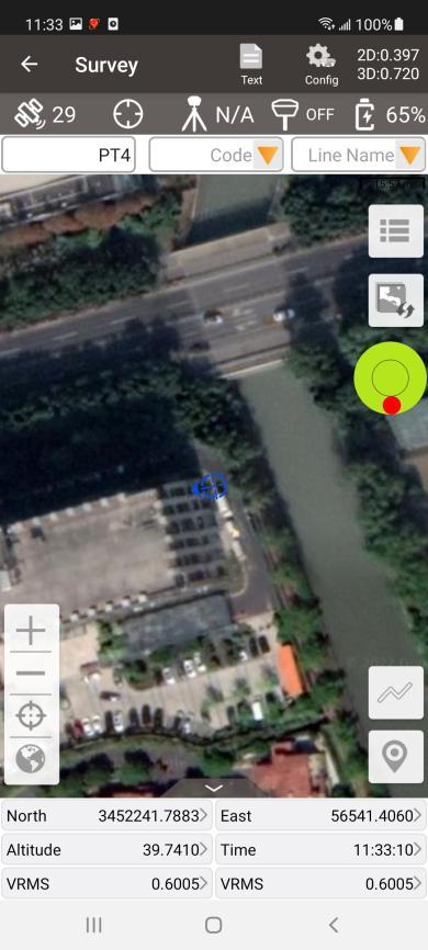
Figure 4.2[]{#_Toc14116 .anchor} Survey -- Drawing mode
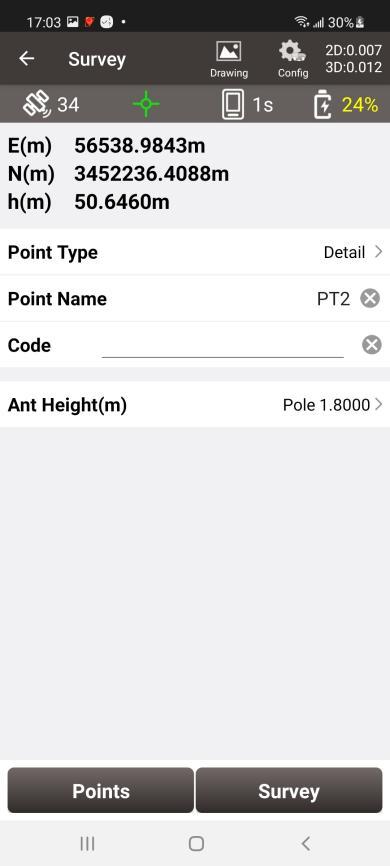
Figure 4.3[]{#_Toc22011 .anchor} Survey -- Text mode
- Status Bar
Icon Description
![]() the main interface is shown in text mode or drawing mode, click this icon to switch between the two modes.
the main interface is shown in text mode or drawing mode, click this icon to switch between the two modes.
![]() Survey Configuration, refer to section 4.6 for more details.
Survey Configuration, refer to section 4.6 for more details.
![]() connection status with a Tersus GNSS receiver, refer to Connect for more details.
connection status with a Tersus GNSS receiver, refer to Connect for more details.
 satellite icon, with the number of satellites involved in solution on the right, e.g., 23 means 23 satellites are used.
 solution status, includes Single, Float
 , Fixed
 , None
 .
.
 data link type, includes Single mode, Base mode
 , Rover UHF mode
 , Rover GSM mode
 , Rover PDA Network mode
 , with the number of Diff Age on the right. If the Diff Age is greater than the Diff Age Limit in survey config, the number is displayed in red.
 tilt status, icons
 ![]()
![]()
![]() all indicate tilt enable but the tilt quality prediction decreases sequentially. The icon
all indicate tilt enable but the tilt quality prediction decreases sequentially. The icon ![]() indicates tilt need to be initialized and the icon
indicates tilt need to be initialized and the icon  indicates tilt is turned OFF. The tilt compensation status shows on the right: ON means the tilt compensation is available, and the accuracy meets the requirements; N/A means the tilt compensation is on, pending initialization; OFF means the tilt compensation is off, click it to jump to open it.
 battery icon, with the number of the remaining battery power of GNSS receiver on the right. Currently it is not supported of displaying the battery of David as there is no embedded battery in David receiver.
 external power icon, indicates that Oscar / Luka is currently powered by an external power supply.
- Input Bar
Icon Description
![]() point name input box, the name for the next survey point; when a duplicate point name is entered, the software allows repeated measurement of the point in the same name; when a name prefix exists is entered, the maximum point name under the prefix will be prompted.
point name input box, the name for the next survey point; when a duplicate point name is entered, the software allows repeated measurement of the point in the same name; when a name prefix exists is entered, the maximum point name under the prefix will be prompted.
![]() code input box, the code for the next survey point. Enter a code or click
code input box, the code for the next survey point. Enter a code or click![]() to select a code in the code list, or search for codes by directly entering code or code summary. When selecting a code for point, such as Fence Post
to select a code in the code list, or search for codes by directly entering code or code summary. When selecting a code for point, such as Fence Post![]() , the next survey point will be used as a point feature; when selecting a code for line, such as EAVE
, the next survey point will be used as a point feature; when selecting a code for line, such as EAVE![]() , then EAVE1 will be entered in the line name box, and the next survey point will be used as a point in the line feature, and the points belonging to the same line name will be connected to form the line.
, then EAVE1 will be entered in the line name box, and the next survey point will be used as a point in the line feature, and the points belonging to the same line name will be connected to form the line.
![]() line name input box, the line name to which the next survey point belongs, enter or click
line name input box, the line name to which the next survey point belongs, enter or click![]() to select a line in the line list. When selecting a code for line, entering or selecting a line, the line survey starts, and the points belonging to the same line name will be connected to form the line.
to select a line in the line list. When selecting a code for line, entering or selecting a line, the line survey starts, and the points belonging to the same line name will be connected to form the line.
- Background Map
+-----------------------------------------------------------------------------------------------------------------------------------------------+-------------------------------------------------------------------------------------------------------------------------------------------------------------------------------------------------------------------------------------------------------------------------------------------------+
| Icon | Description |
+-----------------------------------------------------------------------------------------------------------------------------------------------+-------------------------------------------------------------------------------------------------------------------------------------------------------------------------------------------------------------------------------------------------------------------------------------------------+
| ![]() | view and edit the survey point library. |
+-----------------------------------------------------------------------------------------------------------------------------------------------+-------------------------------------------------------------------------------------------------------------------------------------------------------------------------------------------------------------------------------------------------------------------------------------------------+
|
| view and edit the survey point library. |
+-----------------------------------------------------------------------------------------------------------------------------------------------+-------------------------------------------------------------------------------------------------------------------------------------------------------------------------------------------------------------------------------------------------------------------------------------------------+
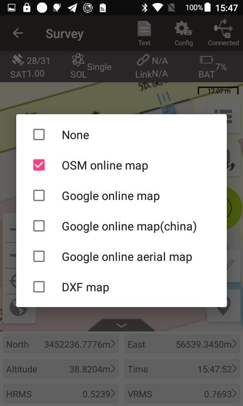
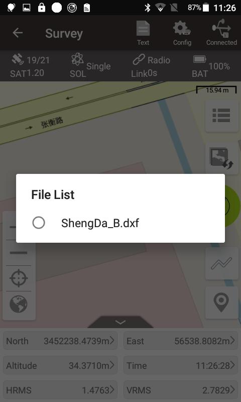
| ![]() | click it to switch among none, OSM online map, Google online map, Google online map (China) and Google online aerial map. |
| | |
| | After importing vactor maps in Import module, or putting vector map files in DXF, LandXML, KML, KMZ format under the file path: internal storage\TersusSurvey\Maps, then you can choose the vector map you want to display in the list besides online map. |
| | |
| | Note: before loading a vector base map, ensure the coordinate system parameters in the current project are consistent with the coordinate system parameters in the vector base map. |
| | |
| | +---------------------------------------------------------------------------------------------------------------------------------------------+---------------------------------------------------------------------------------------------------------------------------------------------+ |
| | |
| click it to switch among none, OSM online map, Google online map, Google online map (China) and Google online aerial map. |
| | |
| | After importing vactor maps in Import module, or putting vector map files in DXF, LandXML, KML, KMZ format under the file path: internal storage\TersusSurvey\Maps, then you can choose the vector map you want to display in the list besides online map. |
| | |
| | Note: before loading a vector base map, ensure the coordinate system parameters in the current project are consistent with the coordinate system parameters in the vector base map. |
| | |
| | +---------------------------------------------------------------------------------------------------------------------------------------------+---------------------------------------------------------------------------------------------------------------------------------------------+ |
| | |  |
|  | |
| | | | | |
| | | Figure 4.4[]{#_Toc23999 .anchor} Map options | Figure 4.5[]{#_Toc6715 .anchor} DXF file list | |
| | +---------------------------------------------------------------------------------------------------------------------------------------------+---------------------------------------------------------------------------------------------------------------------------------------------+ |
| | |
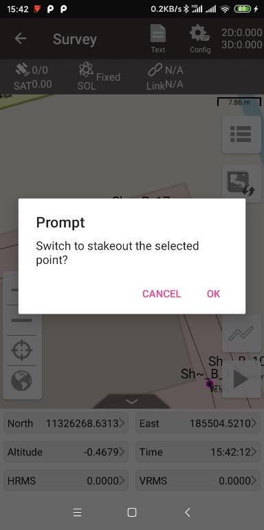
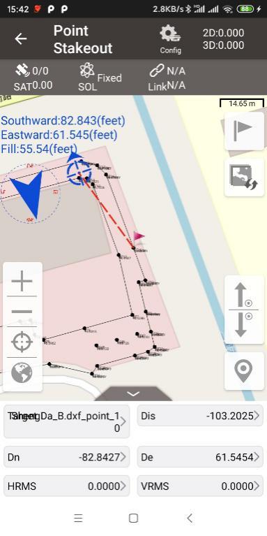
| | After the dxf map is selected, Nuwa app will load the map. Select one point on the DXF base map, it prompts whether to stakeout the selected point. If you click OK, it switches to the point stakeout interface to stakeout this point. |
| | |
| | +----------------------------------------------------------------------------------------------------------------------------------------------+----------------------------------------------------------------------------------------------------------------------------------------------+ |
| | |
| |
| | | | | |
| | | Figure 4.4[]{#_Toc23999 .anchor} Map options | Figure 4.5[]{#_Toc6715 .anchor} DXF file list | |
| | +---------------------------------------------------------------------------------------------------------------------------------------------+---------------------------------------------------------------------------------------------------------------------------------------------+ |
| | |
| | After the dxf map is selected, Nuwa app will load the map. Select one point on the DXF base map, it prompts whether to stakeout the selected point. If you click OK, it switches to the point stakeout interface to stakeout this point. |
| | |
| | +----------------------------------------------------------------------------------------------------------------------------------------------+----------------------------------------------------------------------------------------------------------------------------------------------+ |
| | |  |
|  | |
| | | | | |
| | | Figure 4.6[]{#_Toc27767 .anchor} Prompt to stakeout the point | Figure 4.7[]{#_Toc19376 .anchor} Switch to point stakeout | |
| | +----------------------------------------------------------------------------------------------------------------------------------------------+----------------------------------------------------------------------------------------------------------------------------------------------+ |
| | |
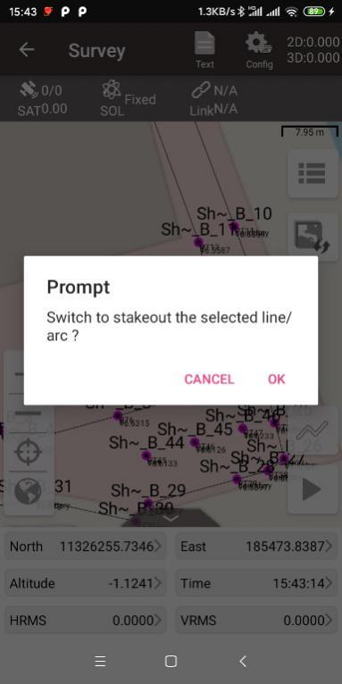
| | Select a line on the DXF base map, it prompts whether to stakeout this line. If you click OK, it switches to the line stakeout interface to stakeout this line. |
| | |
| | +----------------------------------------------------------------------------------------------------------------------------------------------+----------------------------------------------------------------------------------------------------------------------------------------------+ |
| | |
| |
| | | | | |
| | | Figure 4.6[]{#_Toc27767 .anchor} Prompt to stakeout the point | Figure 4.7[]{#_Toc19376 .anchor} Switch to point stakeout | |
| | +----------------------------------------------------------------------------------------------------------------------------------------------+----------------------------------------------------------------------------------------------------------------------------------------------+ |
| | |
| | Select a line on the DXF base map, it prompts whether to stakeout this line. If you click OK, it switches to the line stakeout interface to stakeout this line. |
| | |
| | +----------------------------------------------------------------------------------------------------------------------------------------------+----------------------------------------------------------------------------------------------------------------------------------------------+ |
| | |  |
|  | |
| | | | | |
| | | Figure 4.8[]{#_Toc1842 .anchor} Prompt to stakeout the line | Figure 4.9[]{#_Toc6137 .anchor} Switch to line stakeout | |
| | +----------------------------------------------------------------------------------------------------------------------------------------------+----------------------------------------------------------------------------------------------------------------------------------------------+ |
+-----------------------------------------------------------------------------------------------------------------------------------------------+-------------------------------------------------------------------------------------------------------------------------------------------------------------------------------------------------------------------------------------------------------------------------------------------------+
| |
| | | | | |
| | | Figure 4.8[]{#_Toc1842 .anchor} Prompt to stakeout the line | Figure 4.9[]{#_Toc6137 .anchor} Switch to line stakeout | |
| | +----------------------------------------------------------------------------------------------------------------------------------------------+----------------------------------------------------------------------------------------------------------------------------------------------+ |
+-----------------------------------------------------------------------------------------------------------------------------------------------+-------------------------------------------------------------------------------------------------------------------------------------------------------------------------------------------------------------------------------------------------------------------------------------------------+
Icon Description
![]() zoom in the map.
zoom in the map.
![]() zoom out the map.
zoom out the map.
![]() zoom with the current location at the center.
zoom with the current location at the center.
![]() place all the points in one view.
place all the points in one view.
more features can be added to the screen in Survey Config
- Tools
+------------------------------------------------------------------------------------------------------------------------------------------------------------+------------------------------------------------------------------------------------------------------------------------------------------------------------------------------------------------------------------------------------------------------------------------------------------------------------------------------------------------------------------------------------------------------------------------------------------------------------------------------------------------------------------------------------------------------------------------------------+
| Icon | Description |
+------------------------------------------------------------------------------------------------------------------------------------------------------------+------------------------------------------------------------------------------------------------------------------------------------------------------------------------------------------------------------------------------------------------------------------------------------------------------------------------------------------------------------------------------------------------------------------------------------------------------------------------------------------------------------------------------------------------------------------------------------+
|  | electronic bubble: indicates leveling bubble calibration status. The bubble is blue when it is calibrated to the center inside the black circle, and is red when it is not calibrated to the center circle. |
+------------------------------------------------------------------------------------------------------------------------------------------------------------+------------------------------------------------------------------------------------------------------------------------------------------------------------------------------------------------------------------------------------------------------------------------------------------------------------------------------------------------------------------------------------------------------------------------------------------------------------------------------------------------------------------------------------------------------------------------------------+
|
| electronic bubble: indicates leveling bubble calibration status. The bubble is blue when it is calibrated to the center inside the black circle, and is red when it is not calibrated to the center circle. |
+------------------------------------------------------------------------------------------------------------------------------------------------------------+------------------------------------------------------------------------------------------------------------------------------------------------------------------------------------------------------------------------------------------------------------------------------------------------------------------------------------------------------------------------------------------------------------------------------------------------------------------------------------------------------------------------------------------------------------------------------------+
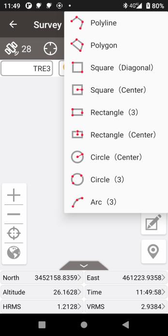
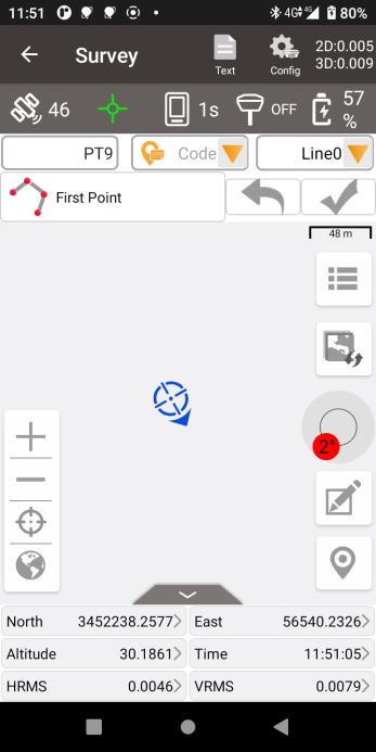
| ![]() | Graphic measurement function: |
| | |
| | After clicking this icon, select the target graphic: polyline, polygon, square, rectangle, circle or arc; enter the line name and click [OK] to start graphic measurement. In the measurement, complete the point survey according to the prompts, the survey points collected will be automatically connected to the selected graphics, and the graphics will be saved in the line list. |
| | |
| | +-------------------------------------------------------------------------------------------------------------------------------+--------------------------------------------------------------------------------------------------------------------------------+ |
| | |
| Graphic measurement function: |
| | |
| | After clicking this icon, select the target graphic: polyline, polygon, square, rectangle, circle or arc; enter the line name and click [OK] to start graphic measurement. In the measurement, complete the point survey according to the prompts, the survey points collected will be automatically connected to the selected graphics, and the graphics will be saved in the line list. |
| | |
| | +-------------------------------------------------------------------------------------------------------------------------------+--------------------------------------------------------------------------------------------------------------------------------+ |
| | |  |
|  | |
| | | | | |
| | | Figure 4.10[]{#_Toc2102 .anchor} Graphic selection | Figure 4.11[]{#_Toc26676 .anchor} Graphic measurement | |
| | +-------------------------------------------------------------------------------------------------------------------------------+--------------------------------------------------------------------------------------------------------------------------------+ |
| | |
| | In the graphic measurement, take a measurement or click to select existing points to form a graphic; click
| |
| | | | | |
| | | Figure 4.10[]{#_Toc2102 .anchor} Graphic selection | Figure 4.11[]{#_Toc26676 .anchor} Graphic measurement | |
| | +-------------------------------------------------------------------------------------------------------------------------------+--------------------------------------------------------------------------------------------------------------------------------+ |
| | |
| | In the graphic measurement, take a measurement or click to select existing points to form a graphic; click![]() , the latest point collected will be undone and no longer used for graphic composition; click
, the latest point collected will be undone and no longer used for graphic composition; click ![]() , to complete or exit the current graphic measurement. |
| | |
| | If Display Survey Line Detail in Survey Config - Display Config is checked, the line segment lengths and polygon areas will be displayed during the graphic measurement. |
| | |
| | If you need to continue measuring a polyline that has already been completed, enter the exist line name of the polyline directly and continue the polyline measurement from start or from end point. |
+------------------------------------------------------------------------------------------------------------------------------------------------------------+------------------------------------------------------------------------------------------------------------------------------------------------------------------------------------------------------------------------------------------------------------------------------------------------------------------------------------------------------------------------------------------------------------------------------------------------------------------------------------------------------------------------------------------------------------------------------------+
|
, to complete or exit the current graphic measurement. |
| | |
| | If Display Survey Line Detail in Survey Config - Display Config is checked, the line segment lengths and polygon areas will be displayed during the graphic measurement. |
| | |
| | If you need to continue measuring a polyline that has already been completed, enter the exist line name of the polyline directly and continue the polyline measurement from start or from end point. |
+------------------------------------------------------------------------------------------------------------------------------------------------------------+------------------------------------------------------------------------------------------------------------------------------------------------------------------------------------------------------------------------------------------------------------------------------------------------------------------------------------------------------------------------------------------------------------------------------------------------------------------------------------------------------------------------------------------------------------------------------------+
| ![]() | When selecting continuous for survey mode, click to start continuous points automatically survey. |
+------------------------------------------------------------------------------------------------------------------------------------------------------------+------------------------------------------------------------------------------------------------------------------------------------------------------------------------------------------------------------------------------------------------------------------------------------------------------------------------------------------------------------------------------------------------------------------------------------------------------------------------------------------------------------------------------------------------------------------------------------+
|
| When selecting continuous for survey mode, click to start continuous points automatically survey. |
+------------------------------------------------------------------------------------------------------------------------------------------------------------+------------------------------------------------------------------------------------------------------------------------------------------------------------------------------------------------------------------------------------------------------------------------------------------------------------------------------------------------------------------------------------------------------------------------------------------------------------------------------------------------------------------------------------------------------------------------------------+
| ![]() | When selecting detail for survey mode, click to start detailed point survey. |
+------------------------------------------------------------------------------------------------------------------------------------------------------------+------------------------------------------------------------------------------------------------------------------------------------------------------------------------------------------------------------------------------------------------------------------------------------------------------------------------------------------------------------------------------------------------------------------------------------------------------------------------------------------------------------------------------------------------------------------------------------+
|
| When selecting detail for survey mode, click to start detailed point survey. |
+------------------------------------------------------------------------------------------------------------------------------------------------------------+------------------------------------------------------------------------------------------------------------------------------------------------------------------------------------------------------------------------------------------------------------------------------------------------------------------------------------------------------------------------------------------------------------------------------------------------------------------------------------------------------------------------------------------------------------------------------------+
| ![]() | When selecting control for survey mode, click to start control point survey. |
+------------------------------------------------------------------------------------------------------------------------------------------------------------+------------------------------------------------------------------------------------------------------------------------------------------------------------------------------------------------------------------------------------------------------------------------------------------------------------------------------------------------------------------------------------------------------------------------------------------------------------------------------------------------------------------------------------------------------------------------------------+
|
| When selecting control for survey mode, click to start control point survey. |
+------------------------------------------------------------------------------------------------------------------------------------------------------------+------------------------------------------------------------------------------------------------------------------------------------------------------------------------------------------------------------------------------------------------------------------------------------------------------------------------------------------------------------------------------------------------------------------------------------------------------------------------------------------------------------------------------------------------------------------------------------+
| ![]() | When selecting control for survey mode, click to choose a control point and start checking survey for the point. |
+------------------------------------------------------------------------------------------------------------------------------------------------------------+------------------------------------------------------------------------------------------------------------------------------------------------------------------------------------------------------------------------------------------------------------------------------------------------------------------------------------------------------------------------------------------------------------------------------------------------------------------------------------------------------------------------------------------------------------------------------------+
| When selecting control for survey mode, click to choose a control point and start checking survey for the point. |
+------------------------------------------------------------------------------------------------------------------------------------------------------------+------------------------------------------------------------------------------------------------------------------------------------------------------------------------------------------------------------------------------------------------------------------------------------------------------------------------------------------------------------------------------------------------------------------------------------------------------------------------------------------------------------------------------------------------------------------------------------+
- Information Bar
Six information items are displayed, each can be chosen from the items in the following screenshots.
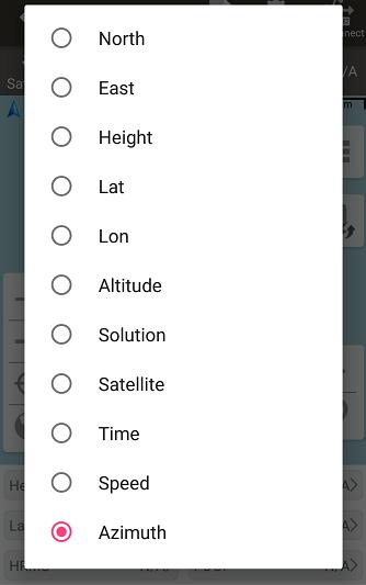
Figure 4.12[]{#_Toc17201 .anchor} Information option list -- part 1
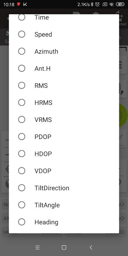
Figure 4.13[]{#_Toc23585 .anchor} Information option list -- part 2
[North]: the North Coordinates of current position.
[East]: the East Coordinates of current position.
[Altitude]: the Altitude of current positon.
[Lat]: the Latitude Coordinates of current position.
[Lon]: the Longitude Coordinates of current position.
[Height]: the ellipsoidal height of current position.
[Solution]: the status of RTK, including fixed, float, single, etc.
[Time]: current time.
[Speed]: current speed.
[Compass]: the azimuth of the controller.
[Ant.H]: the height of the receiver.
[RMS]: root mean square, precision indicators.
[DOP]: dilution of precision, the spatial geometric distribution of satellites.
[Target]: the name of the target in stakeout.
[Dn]: the distance between current position and the target in North direction.
[De]: the distance between current position and the target in East direction.
[Dh]: the difference in height between current position and the target.
[Offset]: the distance between current position and the target.
[Miles]: the miles of the target, from the start of the line.
[Remain miles]: the remain miles to the end of the line.
[TiltDirect]: the azimuth of tilt direction.
[TiltAngle]: the angle of tilt.
[Heading]: the heading of the receiver.
[Dis to Last]: the distance from the last survey point.
[Dis to Base]: the distance to Base reference station.
Point Stakeout
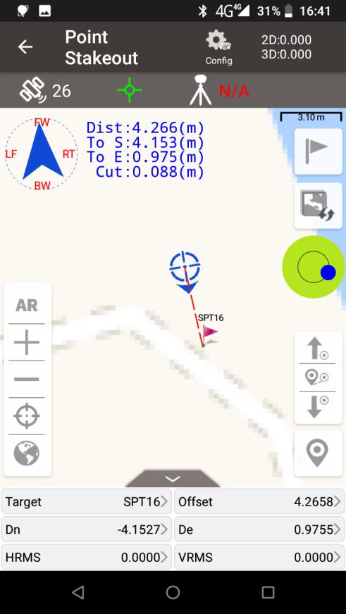
Figure 4.14[]{#_Toc31100 .anchor} Point Stakeout interface
The above screenshot is the main interface of point stakeout, which is similar to that of point survey.
The main steps of point stakeout are as follows:
-
Add stakeout point: click
 to enter the stakeout point library which is shown in Figure 4.15 below, refer to section 0 for point library management.
 -
Select the point to be stakeout: select the point, then click [Select].
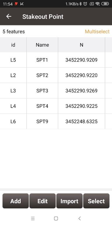
Figure 4.15[]{#_Toc131 .anchor} Add stakeout point
-
The offset between the current point and the target point is displayed on the screen. The arrow icons
 and
and  are used to switch the stakeout points in the library. The icon
 is used to switch to the nearest stakeout points in the library.
 -
If the display all staking point and point name are checked in Survey Config - Display Config, directly clicking on the point to be stake on the map can also used to switch the staking points.
In the point stakeout interface,
-
The red flag indicates the location of the stakeout point.
-
The red dotted line is the connection between the current point and the point to be staked.
-
The small blue arrow is the point to be staked.
-
The small blue arrow pointing towards the surveyor heading.
-
The big blue arrow prompts the surveyor that the point to be staked is in the front/rear/left/right position.
-
The blue number shows the distance from the point to be staked in different directions.
<!-- -->
-
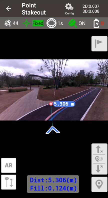
After selecting the staking target, the icon
 is used to open AR mode.
If the connected device such as TS20 or TS21 that are equipped with stakeout cameras, the cameras will be activated to overlay the target point, along with the direction and distance to the target, on the live view. When the distance to the target is relatively far, the front camera is used to display the AR stakeout view; as the user approaches the target, it will switch to the bottom camera automatically to provide a more accurate AR stakeout view.
+----------------------------------------------------------------------------------------------------------------------------------+---------------------------------------------------------------------------------------------------------------------------------------------+
|  |
| 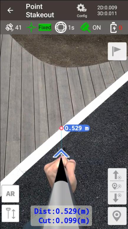 |
| | |
| Figure 4.16[]{#_Toc25504 .anchor} Front caemra AR stakeout | Figure 4.17[]{#_Toc17610 .anchor} Bottom camera AR stakeout |
+----------------------------------------------------------------------------------------------------------------------------------+---------------------------------------------------------------------------------------------------------------------------------------------+
|
| | |
| Figure 4.16[]{#_Toc25504 .anchor} Front caemra AR stakeout | Figure 4.17[]{#_Toc17610 .anchor} Bottom camera AR stakeout |
+----------------------------------------------------------------------------------------------------------------------------------+---------------------------------------------------------------------------------------------------------------------------------------------+
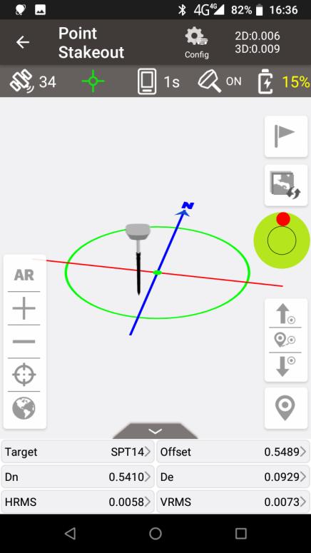
If the connected device does not have a stakeout camera, Nuwa will use the controller camera to display the direction and distance to the target on the live scene; and when approaching the target point, Nuwa switches to a 3D display to show the relative positional relationship between the current pole tip and the target point.
+-----------------------------------------------------------------------------------------------------------------------------------------------------------------------+-----------------------------------------------------------------------------------------------------------------------------------------------------------------------+
| 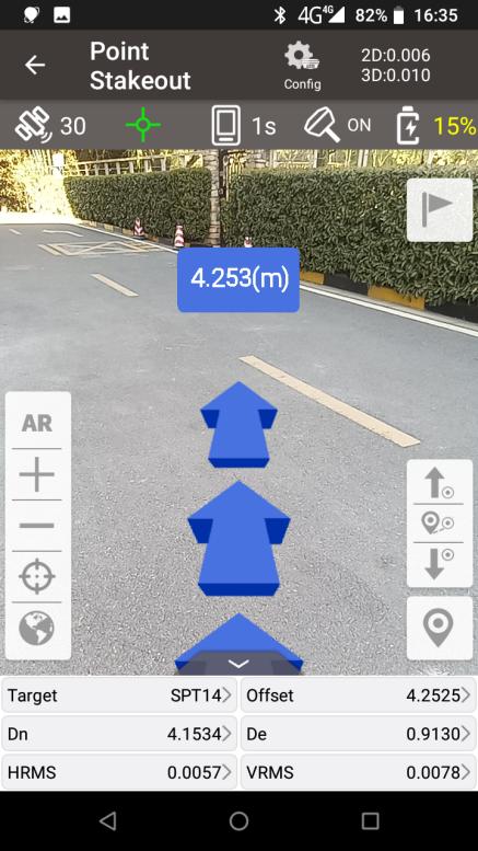 |
|  |
| | |
| Figure 4.18[]{#_Toc28991 .anchor} Controller Camera AR stakeout | Figure 4.19[]{#_Toc10706 .anchor} 3D display |
+-----------------------------------------------------------------------------------------------------------------------------------------------------------------------+-----------------------------------------------------------------------------------------------------------------------------------------------------------------------+
|
| | |
| Figure 4.18[]{#_Toc28991 .anchor} Controller Camera AR stakeout | Figure 4.19[]{#_Toc10706 .anchor} 3D display |
+-----------------------------------------------------------------------------------------------------------------------------------------------------------------------+-----------------------------------------------------------------------------------------------------------------------------------------------------------------------+
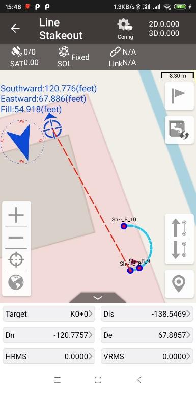
Line Stakeout
There are four circumstances of line stakeout: straight line stakeout, polyline stakeout, arc stakeout, and circle stakeout.
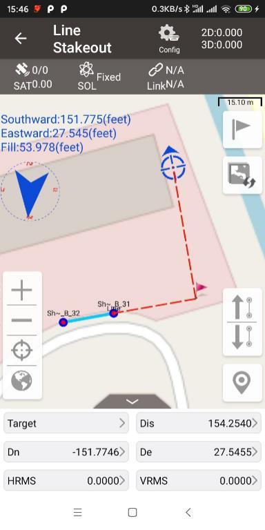
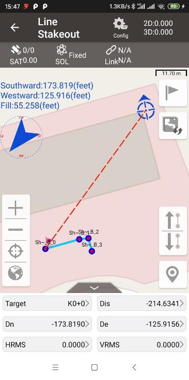
(1) Straight line stakeout
Click ![]() to enter stakeout line library, plot the staking line on the map, and the software will mark the target point and the direction of the staking line directly according to the staking properties of the staking line (stake to pile interval or stake to vertical point).
to enter stakeout line library, plot the staking line on the map, and the software will mark the target point and the direction of the staking line directly according to the staking properties of the staking line (stake to pile interval or stake to vertical point).
+----------------------------------------------------------------------------------------------------------------------------------------------+----------------------------------------------------------------------------------------------------------------------------------------------+
|  |
|  |
| | |
| Figure 4.20[]{#_Toc14171 .anchor} Configure straight line stakeout | Figure 4.21[]{#_Toc13473 .anchor} Stakeout a straight line |
+----------------------------------------------------------------------------------------------------------------------------------------------+----------------------------------------------------------------------------------------------------------------------------------------------+
|
| | |
| Figure 4.20[]{#_Toc14171 .anchor} Configure straight line stakeout | Figure 4.21[]{#_Toc13473 .anchor} Stakeout a straight line |
+----------------------------------------------------------------------------------------------------------------------------------------------+----------------------------------------------------------------------------------------------------------------------------------------------+
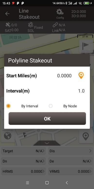
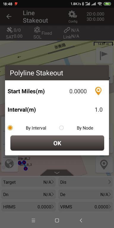
(2) Polyline stakeout
Select to stake out to the pile point, to the node or to the nearest point on the polyline. Stake out to the pile point starts from the beginning of the polyline according to the pile interval, but stops at the node; stake out to the node will directly stake out the end points of each line segment of the polyline. Stake out to the points on the offset line by entering the offset value.
+----------------------------------------------------------------------------------------------------------------------------------------------+----------------------------------------------------------------------------------------------------------------------------------------------+
|  |
|  |
| | |
| Figure 4.22[]{#_Toc29971 .anchor} Configure polyline stakeout | Figure 4.23[]{#_Toc21662 .anchor} Stakeout a polyline |
+----------------------------------------------------------------------------------------------------------------------------------------------+----------------------------------------------------------------------------------------------------------------------------------------------+
|
| | |
| Figure 4.22[]{#_Toc29971 .anchor} Configure polyline stakeout | Figure 4.23[]{#_Toc21662 .anchor} Stakeout a polyline |
+----------------------------------------------------------------------------------------------------------------------------------------------+----------------------------------------------------------------------------------------------------------------------------------------------+
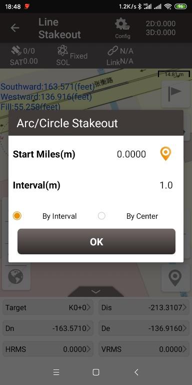
(3) Arc stakeout
Select to stake out to the pile point, to the center of a circle or to the nearest point on the arc. Stake out to the pile point is to stake out sequentially from the starting point of the polyline according to the pile interval; stake out to the circle center is to stake out directly to the center of this arc.
+----------------------------------------------------------------------------------------------------------------------------------------------+----------------------------------------------------------------------------------------------------------------------------------------------+
|  |
|  |
| | |
| Figure 4.24[]{#_Toc30383 .anchor} Configure arc stakeout | Figure 4.25[]{#_Toc25443 .anchor} Stakeout an arc |
+----------------------------------------------------------------------------------------------------------------------------------------------+----------------------------------------------------------------------------------------------------------------------------------------------+
|
| | |
| Figure 4.24[]{#_Toc30383 .anchor} Configure arc stakeout | Figure 4.25[]{#_Toc25443 .anchor} Stakeout an arc |
+----------------------------------------------------------------------------------------------------------------------------------------------+----------------------------------------------------------------------------------------------------------------------------------------------+
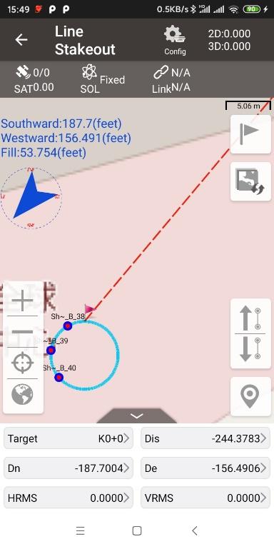
(4) Circle stakeout
Select to stake out to the pile point, to the center of a circle or to the nearest point on the circle. Stake out to the pile point is to stake out clockwise from the northernmost point on the circle according to the pile interval; stake out to the circle center is to stake out directly to the center of this circle.
+----------------------------------------------------------------------------------------------------------------------------------------------+----------------------------------------------------------------------------------------------------------------------------------------------+
| |  |
| | |
| Figure 4.26[]{#_Toc5920 .anchor} Configure arc stakeout | Figure 4.27[]{#_Toc24584 .anchor} Stakeout a circle |
+----------------------------------------------------------------------------------------------------------------------------------------------+----------------------------------------------------------------------------------------------------------------------------------------------+
|
| | |
| Figure 4.26[]{#_Toc5920 .anchor} Configure arc stakeout | Figure 4.27[]{#_Toc24584 .anchor} Stakeout a circle |
+----------------------------------------------------------------------------------------------------------------------------------------------+----------------------------------------------------------------------------------------------------------------------------------------------+
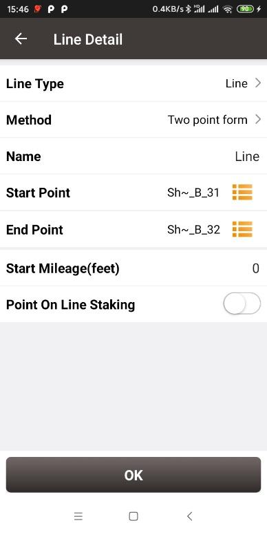
In the above screenshot of line detail,
[Line Type]: line is the only line type currently.
[Method]: two methods to add a stakeout line, details refer to section 2.5.1.
[Name]: the line name can be modified manually.
[Start Mileage]: the mileage at the starting point, used to calculate mileage at subsequent points.
[Point On Line Staking]: when this button is turned on, stake out points on the line (or offset line) according to the entered Interval and Offset; when this button is turned off, stake out directly to the line, that is, stake out to the vertical cross point of the current position and the selected line.
[Stakeout Interval (m)]: the interval distance of the points on the stakeout line, which means stake out a point every certain distance.
[Offset (m)]: the offset when staking out the points on the stakeout line. When it is negative, it is to the left of the line forward direction. When it is positive, it is to the right of the line forward direction.
-
Select the stakeout line, click [Select].
-
Stake out from the starting point (+ offset), stake out the next point every interval distance. The distance from the current position to the target position will be displayed on the screen
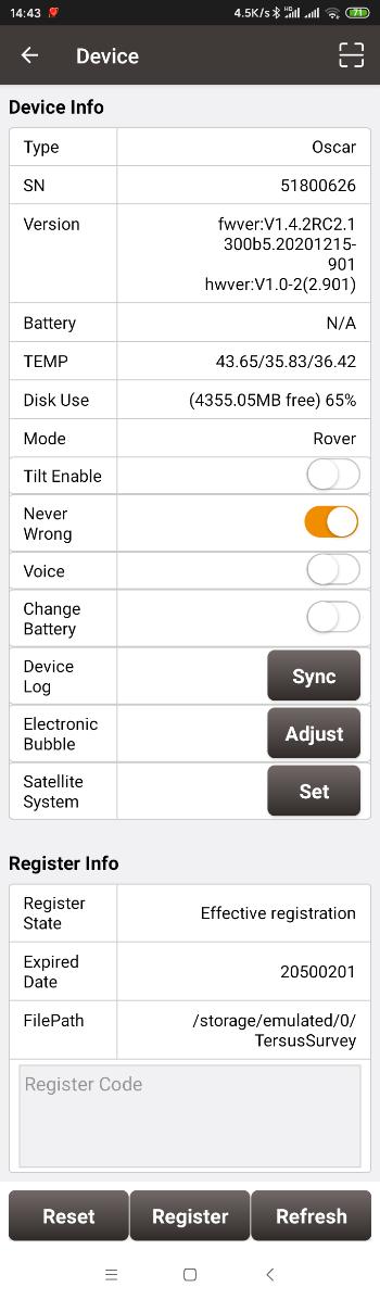
Tilt Survey and Stakeout
Tilt function is only applicable for Oscar GNSS receiver Ultimate version, Luka GNSS receiver Ultimate version and Luka GNSS receiver Advanced version.
Tilt Initialization
The tilt compensation is free of calibration. The tilt compensation will be initialized when the surveyor walks forward naturally for several meters after the receiver gets RTK fixed solution status. You can start tilt survey right after you walk to the survey point.
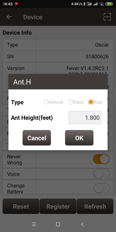
There are two methods to turn on or off tilt compensation. One is turning on or off tilt compensation on Device Info on the OLED via buttons. Another method is through Nuwa app. After the receiver is connect in Nuwa app, and it is configured working as a Rover. Turn on the [Tilt Enable] on the device interface, or click in the Survey interface to turn on the tilt compensation, and then confirm the antenna height.
+--------------------------------------------------------------------------------------------------------------------------------------------+----------------------------------------------------------------------------------------------------------------------------------------------+
|  |
|  |
| | |
| Figure 4.28[]{#_Toc32735 .anchor} Enable Tilt in device info | Figure 4.29[]{#_Toc32357 .anchor} Setting antenna height when enabling tilt compensation |
+--------------------------------------------------------------------------------------------------------------------------------------------+----------------------------------------------------------------------------------------------------------------------------------------------+
|
| | |
| Figure 4.28[]{#_Toc32735 .anchor} Enable Tilt in device info | Figure 4.29[]{#_Toc32357 .anchor} Setting antenna height when enabling tilt compensation |
+--------------------------------------------------------------------------------------------------------------------------------------------+----------------------------------------------------------------------------------------------------------------------------------------------+
When tilt function is enabled, the tilt LED on the receiver OLED display lights on with steady red. When the solution status is single, it flashes red. When the solution status is RTK float, or the solution status is RTK fixed while tilt compensation is invalid, it changes to flashing green. When RTK solution status is fixed and the tilt compensation is available, the tilt LED turns steady green.
When the tilt compensation is valid, click in the Survey interface to view the detailed information of tilt compensation including tilt status, tilt direction, tilt angle, heading and their quality index. Among them, the tilt direct indicates which direction is tilted, that is, the angle between the projection of the ranging pole on the ground and the north direction after tilting; the tilt angle indicates the degree of tilt, that is, the angle between the tilted pole and the vertical direction; Heading indicates the surveyor's orientation (the facing of the back of the receiver, we consider the panel of the receiver is always facing the surveyor).
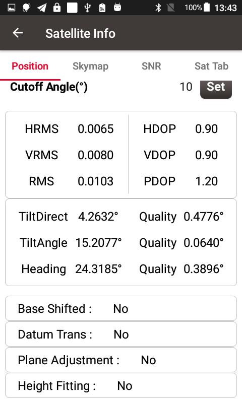
Figure 4.30[]{#_Toc14126 .anchor} Detailed information of tilt compensation
Tilt Survey
After turning on [Tilt Enable] and tilt initialization is finished, enter Survey interface and start tilt survey.
The tilt status is displayed at the top of the survey interface. When the tilt status is ON, it is considered that the tilt compensation accuracy is high and it is in a usable state. You can start survey using the tilted ranging pole. Please ensure that the antenna height setting is correct which will affect the tilt measurement results.
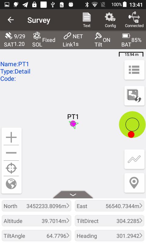
Figure 4.31[]{#_Toc18297 .anchor} Tilt status is ON
When the status is displayed as N/A and blinking, it is considered that the accuracy of tilt compensation is reduced and it is in a state that is not recommended. At this time, the tilt indicator of the receiver OLED display turns flashing green. This may be caused by the surveyor standing for too long, rotating the ranging pole, or hitting the ranging pole to the ground. When the status is N/A, you need to redo the initialization. Generally, you do not need to stand still, just hold the ranging pole and walk forward to the next point, the initialization is complete automatically.
Note: during the tilt survey, please keep the receiver OLED display facing the surveyor as much as possible. Please do not rotate the pole or hit the pole to the ground, which will invalidate the initialization or affect the accuracy of the tilt compensation. In addition, during the tilt point survey, if it does not continue at the third epoch reached when it is set smoothing 5 epochs for surveying points, please check whether the tilt compensation is invalid. It is not allowed to continue to complete the survey in the case where the tilt initialization accuracy is low.
Tilt Stakeout
After turning on [Tilt Enable] and tilt initialization is finished, enter the Point Stakeout or Line Stakeout interface can start tilt stakeout. The tilt state is also added at the top of the stakeout interface to indicate the current tilt available state.
During the tilt stakeout process, if you enter the threshold range of the stakeout setting, the software will display a virtual tilt ranging pole along with the beep sounds. It is drawn according to the tilt direction angle. When the pole is tilted in a certain direction among east, west, south and north, the virtual tilt ranging pole on the interface will also tilt in a certain direction.
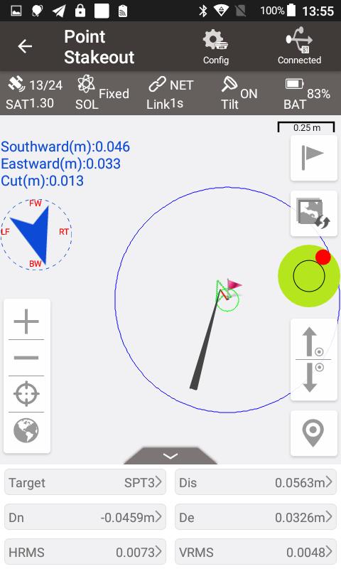
Figure 4.32[]{#_Toc5615 .anchor} Point stakeout when tilt compensation is on
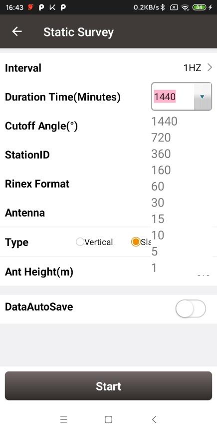
Static Survey
+-----------------------------------------------------------------------------------------------------------------------------------+----------------------------------------------------------------------------------------------------------------------------------------------+
|  |
|  |
| | |
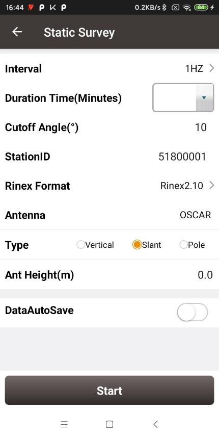
| Figure 4.33[]{#_Toc12997 .anchor} Static Survey interface | Figure 4.34[]{#_Toc14218 .anchor} Duration options |
+-----------------------------------------------------------------------------------------------------------------------------------+----------------------------------------------------------------------------------------------------------------------------------------------+
|
| | |
| Figure 4.33[]{#_Toc12997 .anchor} Static Survey interface | Figure 4.34[]{#_Toc14218 .anchor} Duration options |
+-----------------------------------------------------------------------------------------------------------------------------------+----------------------------------------------------------------------------------------------------------------------------------------------+
[Interval]: selected from 20HZ, 10HZ, 5HZ, 1HZ, 5S, 10S, 15S, 30S and 60S.
[Duration Time (Minutes)]: static survey duration, the recording time can be selected in the drop down list or typed manually.
[Cutoff Angle]: the elevation mask angle, usually set to 15°.
[StationID]: the name of the surveying station.
[Rinex Format]: selected from Rinex2.10, Rinex3.02, and NONE.
[Antenna]: the antenna type.
[Type]: selected from vertical, slant or pole.
[Ant Height]: the height of the antenna.
[Record Antenna Type]: the default is off, which means the antenna type will be not recorded and the antenna height will be recorded as the height of phase center in Rinex header; when on, the antenna type will be recorded and the antenna height will be recorded as the height of the bottom of receiver in Rinex header.
[DataAutoSave]: if this function is turned on, when the static recording time reaches the set duration, the receiver closes the current file record, reopens a file to continue recording, and this cycles; the receiver will also reopen a file to continue recording static when restart. If this function is turned off, the receiver will stop static recording when the recording time reaches the set duration.
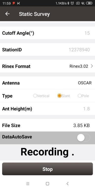
Figure 4.35[]{#_Toc28260 .anchor} Static data recording
After all the parameters are confirmed, click [Start] to start data collection. The static data is recording as shown in the above figure.
Note: Static Survey and Device Debug cannot be used at the same time. Please turn off Device Debug as shown in Figure 3.53 manually before recording static data.
Static data download and post-processing
Static data download for David
Device preparation
-
A David GNSS receiver
-
A DC-2pin to USB power cable
-
A COMM2-7pin to USB & DB9 cable
-
A power bank
-
A computer running TersusDownload tool
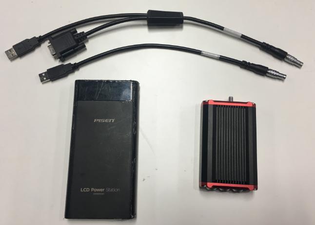
Figure 4.36[]{#_Toc19368 .anchor} Preparation for Static Data Process
After the static survey in fields is completed, connect the David receiver to the computer according to the following figure and power on the David receiver. The USB port is mapped to a serial port (COM5 in the following example) in the computer, which can be checked in the Device Manager.
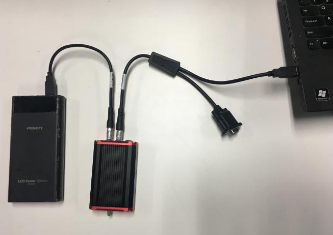
Figure 4.37[]{#_Toc10257 .anchor} Connections of David, computer and power bank
It is recommended to type UNLOGALL in the command window of Tersus GNSS Center software before executing below steps. Open the TersusDownload on the computer, select the serial port to communicate with the David receiver.
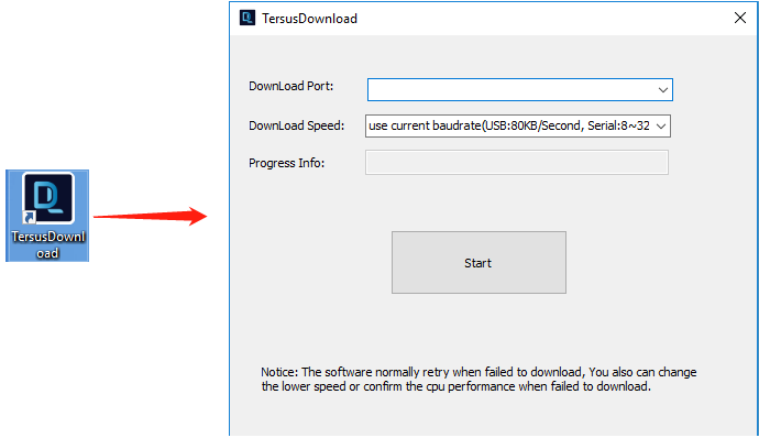
Figure 4.38[]{#_Toc4494 .anchor} TersusDownload interface
Select the download speed. Select 'use current baudrate' when using USB port to download files as shown below. Select baud rate 460800bps if a serial port is used to download files.

Figure 4.39[]{#_Toc3946 .anchor} Download speed options
After completing the above steps, click [Start] and it pops out below window. Select the DownloadPath, select the files to be downloaded, click [Download] to start downloading:
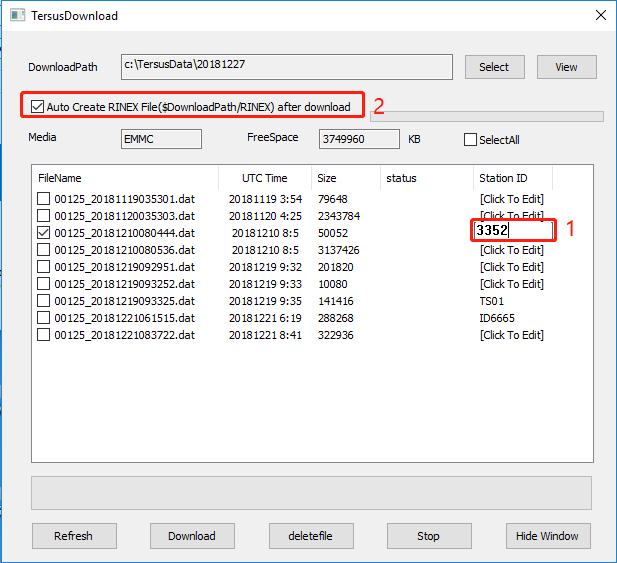
Figure 4.40[]{#_Toc23783 .anchor} File selected for download
In this interface, click the number in red box 1 to edit Station ID if necessary, or it can be edited in Figure 4.31 in section 4.4 Static Survey. Check the box in the left of red box 2 to enable or disable auto create RINEX file after download.
[!] The downloading rate is about 2MB/min, the downloading time can be estimated based on it.
[!] It is recommended to ensure the computer has available CPU and memory when downloading files.
Open the RINEX file using notepad or other text viewing software, the antenna height is vertical height which is from the phase center of the antenna to the point on the ground. The value of the antenna height can be found as shown below.
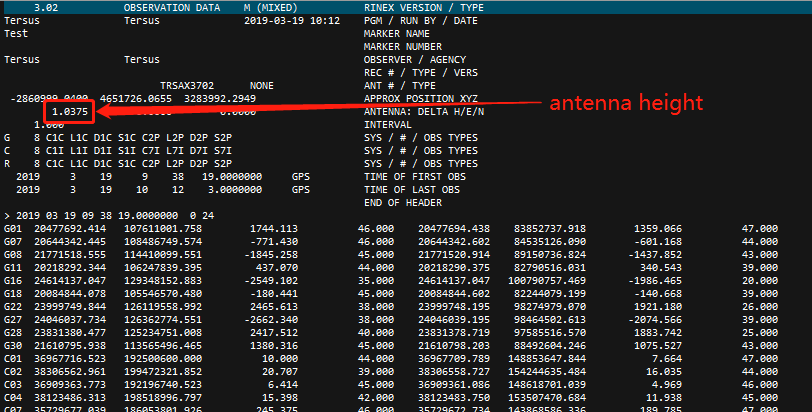
Figure 4.41[]{#_Toc30080 .anchor} View antenna height in the RINEX file
4.5.2 Static data download for Oscar / Luka
Device preparation
-
An Oscar GNSS receiver or a Luka GNSS receiver
-
A mini USB cable for Oscar or a Type-C cable for Luka
-
A computer running RinexConverter tool
Before connecting Oscar / Luka to a computer, ensure the receiver is powered on. Use the Mini USB Cable in the package to connect Oscar to the USB port of a computer, or use the Type-C cable to connect Luka to the USB port of computer, which is shown as below.
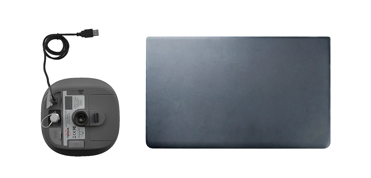
Figure 4.42[]{#_Toc26737 .anchor} Connect Receiver to a computer
After completing the connection, the computer prompts a USB device, open it to view the files as below. Copy the folders and paste them to the computer.

Figure 4.43[]{#_Toc21806 .anchor} Static data recorded by Receiver
Note: When configuring static survey, if configure using buttons only, or configure using Nuwa with selecting None for Rinex format, the receiver only records trs format files. It is necessary to convert trs files to Rinex files before data post-processing.
Open Tersus Rinex Converter software, choose source file path, save path, source format, Rinex version, and click [Process] to complete the format conversion.
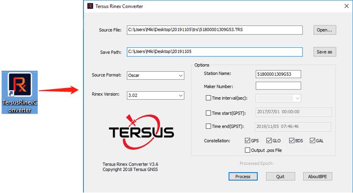
Figure 4.44[]{#_Toc16630 .anchor} Tersus Rinex Converter interface
The Rinex files can be found in the save path as below.
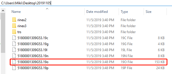
Figure 4.45[]{#_Toc13737 .anchor} The Rinex files after conversion
4.5.3 Data post-processing
Open TERSUS Geo Office software:
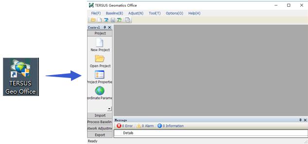
Figure 4.46[]{#_Toc23678 .anchor} TERSUS Geomatics Office interface
After a project is created, click [Import] -> [Import Files]
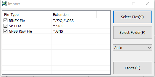
Figure 4.47[]{#_Toc6999 .anchor} Import Files in TERSUS Geo Office
Click [Select Files] to load the Rinex files created in section 7.2.2.
After the above step of importing, the default configuration of the observation data is correct. There is no need to modify the configurations of antenna height, antenna type, and etc. The default configuration of the imported files is shown as follows.
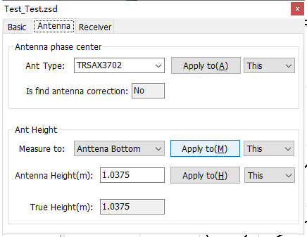
Figure 4.48[]{#_Toc12739 .anchor} Default configuration of the observation data
Refer to the user manual of Tersus Geo Office for more details on data post processing.
Site Calibration
Site Calibration is to find the mathematical conversion relationship (transition parameter) between WGS84 and the local plane Cartesian coordinate system. Site calibration includes the calculation of four-parameter plane transformation and the calculation of height fitting parameters.
After adding point pairs or importing point pairs, select the calculation method. If it is a point pair used for horizontal and vertical calculations, check both H and V. If it is a point pair only for horizontal, just check H; and if it is a point pair only for vertical, just check V.
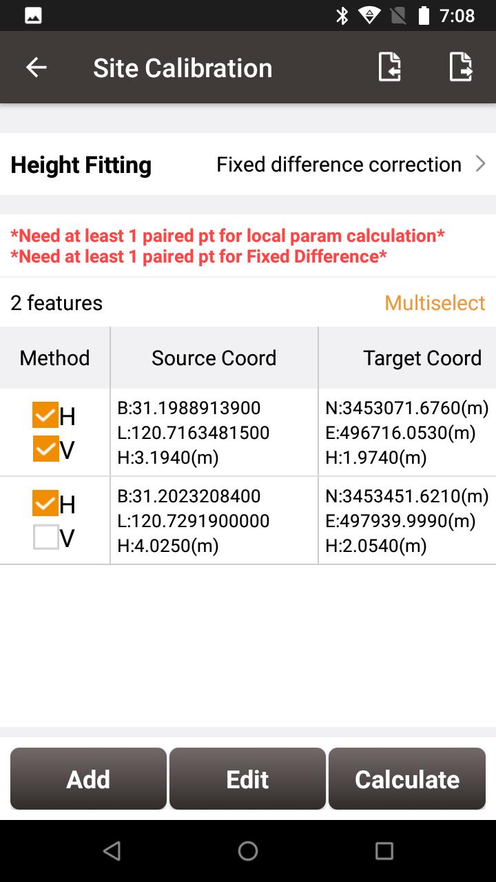
Figure 4.49[]{#_Toc31461 .anchor} Calculation Type options
There are three methods for height-fitting: fixed difference correction, plane fitting and surface fitting, which require 1, 3 and 6 point pairs for vertical calculations.
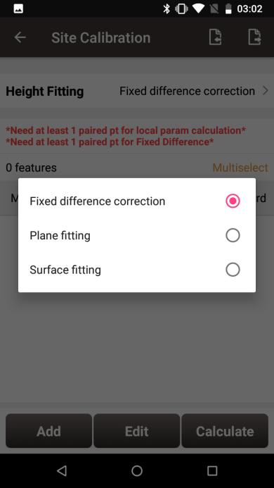
Figure 4.50[]{#_Toc25573 .anchor} Height Fitting options
This section introduces an example of a calculation with one point pair for horizontal and vertical calculations and another point pair only for horizontal calculation.
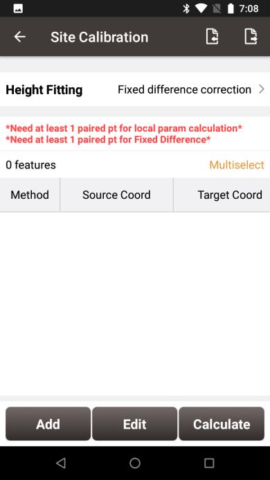
Figure 4.51[]{#_Toc25236 .anchor} Application example for site calibration
Click [Add] to add point for source coordinate and target coordinate.
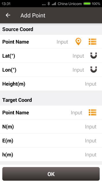
Figure 4.52[]{#_Toc22111 .anchor} Add point for site calibration
The source coordinate can be typed manually or obtained by clicking ![]() the location icon or imported from the survey point library by clicking
the location icon or imported from the survey point library by clicking ![]() the list icon.
the list icon.
The target coordinate can be typed manually or imported from the control point library by clicking ![]() the list icon.
the list icon.
In this example, two pairs of points are type manually for calculation, which are shown below.
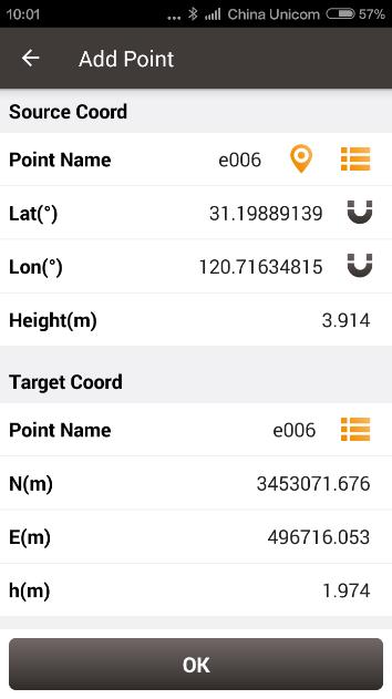
Figure 4.53[]{#_Toc19923 .anchor} The 1^st^ pair of points for calculation

Figure 4.54[]{#_Toc15674 .anchor} The 2^nd^ pair of points for calculation
Click [OK] and two pairs of points are shown below. The first point pair is for horizontal and vertical, and the second is for horizontal.
Figure 4.55[]{#_Toc22291 .anchor} Two pairs of points for calculation
Click [Calculate] and the data is calculated with the result shown below.
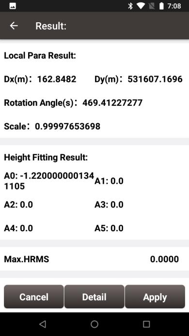
Figure 4.56[]{#_Toc32128 .anchor} Calculation Result
Click [Apply] to apply the site calibration result to the current project coordinate system, and it prompts that 'Apply result successfully!'.
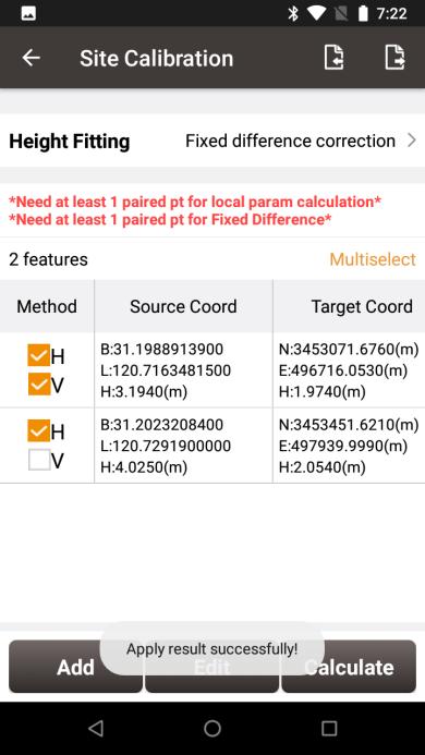
Figure 4.57[]{#_Toc15319 .anchor} Site calibration results applied to current project
Slide left of the title bar to view the values of Residual results as shown below. Since there are not enough point pairs to provide redundant observations in this example, the residual value is 0.
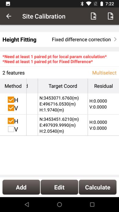
Figure 4.58[]{#_Toc29172 .anchor} Slide left to view residual results
The results applied to the current project coordinate system can be checked in Project Property interface below.
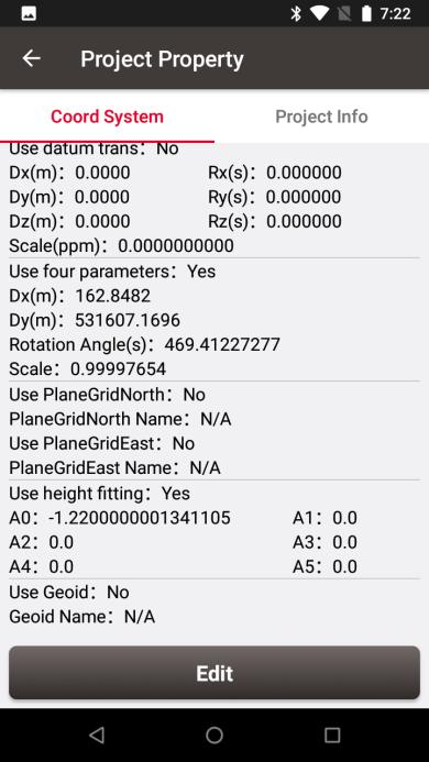
Figure 4.59[]{#_Toc26378 .anchor} Updated project property after site calibration
Survey Config
During data collection, restrictions are given to solution type and HRMS limits, hence only the data meeting the restrictions can be saved. More details are as follows:
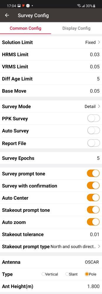
4.7.1 Common Config
+---------------------------------------------------------------------------------------------------------------------------------------------------------------+----------------------------------------------------------------------------------------------------------------------------------------------------------------------------+
|  |
|  |
| | |
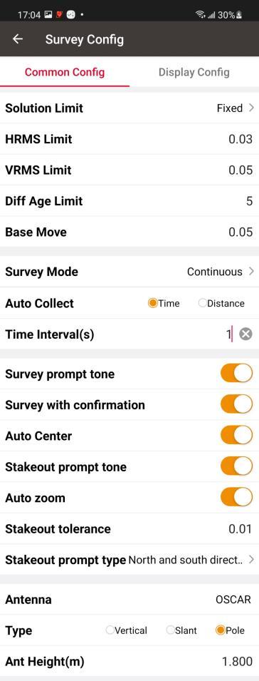
| Figure 4.60[]{#_Toc26624 .anchor} Survey Config - Detail | Figure 4.61[]{#_Toc30102 .anchor} Survey Config -- Continuous |
+---------------------------------------------------------------------------------------------------------------------------------------------------------------+----------------------------------------------------------------------------------------------------------------------------------------------------------------------------+
|
| | |
| Figure 4.60[]{#_Toc26624 .anchor} Survey Config - Detail | Figure 4.61[]{#_Toc30102 .anchor} Survey Config -- Continuous |
+---------------------------------------------------------------------------------------------------------------------------------------------------------------+----------------------------------------------------------------------------------------------------------------------------------------------------------------------------+
[Solution Limited]: includes Single, DGPS, SBAS, Float and Fixed. The solution accuracy (from high to low) is: Fixed > Float > SBAS > DGPS > Single. Select different solution limits, the default HRMS, VRMS limit will change accordingly.
[HRMS Limited]: horizontal RMS limit. Data would not be collected if its HRMS is greater than this limit.
[VRMS Limited]: vertical RMS limit. Data would not be collected if its VRMS is greater than this limit.
[Diff Age Limited]: when the solution status is not single, no data will be collected if the current differential delay exceeds this threshold.
[Base Move]: If the base moves over this limit, there will be a new base point and the rover coordinates will be recalculated according to the new base.
[Survey Mode]: can be selected from detail, continuous and control.
- Detail Point
[PPK Survey]: as known as Stop and Go survey mode, the high-precision position of the rover is obtained by post-processing. The steps are as follows.
a. Start recording Rinex files for base, as the static data of the base for post-processing.
b. Start recording Rinex files for Rover, as the kinematic data of the rover for post-processing. Otherwise, in the subsequent steps, Nuwa will prompt to start the Rinex file recording and jump to the relevant page.
c. Enter the survey configuration interface, open the PPK survey, and set the survey epochs appropriately.
d. Enter the survey interface, start to move the antenna. When reaching the point of interest, stop the antenna, then click the survey button. Enter the name of the point of interest and confirm the antenna value, and click OK to wait for the survey to be completed. Then continue to move the antenna to the next point of interest.
e. When all Stop and Go measurements are completed, stop the Rinex file recording. Copy the two Rinex files to the Windows desktop and import them to the TGO post-processing software.
f. The TGO software will automatically distinguish the static file of the base and the kinematic file of the rover, as well as the points of interest, and form a baseline. Click to process the baseline to calculate the points of interest and generate the PPK processing report.
\[Auto Survey\]: the auto survey can be turned on when PPK survey is on. The survey will be started automatically when reaching the point of interest and centering the bubble.
[Report File]: the report file function can be turned on, the coordinate of the survey epoch will be saved as a .txt file under project folder.
[Survey Epochs]: the survey epoch can be modified. The survey epoch can be positive integer such as 2, 3, 5 or 10. Normally set to 5s.
- Continuous Point
[Auto Collect]: the data can be collected according to Time or Distance.
If Time is selected, ensure to input the time interval.
If Distance is selected, ensure to input the distance interval.
-
Control Point
There are three modes in control point survey, the horizontal and vertical control point, the horizontal control point and the vertical control point.
[Reset Count]: can be modified, and can be any positive integer. The default setting is 2, which means once RTK reset will be performed after starting to collect control points. If the setting is 3, twice RTK reset will be performed after starting.
[Repeat Count]: can be modified, and can be any positive integer. The default setting is 2, which means 2 measurements will be performed after each RTK reset and re-fixed.
[Survey Epochs]: can be modified, and can be any positive integer. The default value is 10, which means that 10 epochs will be observed for each measurement.
[H Diff Limit]: can be modified, as the maximum difference in plane coordinates of the measurements. During the procedure, if the difference exceeds, the procedure will be aborted.
[V Diff Limit]: can be modified, as the maximum difference in elevation coordinates of the measurements. During the procedure, if the difference exceeds, the procedure will be aborted.
[H Diff Check]: can be modified, as the maximum horizontal difference between check point and the selected control point. During the check point survey procedure, if the difference exceeds, the procedure will be aborted.
[V Diff Check]: can be modified, as the maximum vertical difference between check point and the selected control point. During the check point survey procedure, if the difference exceeds, the procedure will be aborted.
[Report File]: the report file function can be turned on, the difference between each epoch and final average result will be saved as a HTML report under project folder.
[Record Base Point]: the record base point function can be turned on, which will save the new base point to the point database before the control point measurement starts and after RTK reset.
-
Offset Point
There are three modes in offset point survey, the tilt offset method, the two point method and the one point method. After selecting the survey mode as offset survey, return to the survey interface to select the method of offset point survey.
[Tilt Offset]: The offset point is calculated from the bottom position of the tilt pole and the entered offset value, which is in the opposite direction to the current tilt direction.
[Two Point Method]: The direction is determined by the two measured points and the offset point is calculated from the second point and the entered offset value.
[One Point Method]: The offset point is calculated from the current position, the entered direction azimuth and offset value.
[Name Increment]: can be modified, the point name will be automatically increased according to the set name increment.
[Survey Prompt Tone]: can be enable or disabled.
[Survey with confirmation]: When it is turned on, the confirmation dialog box will pop up when a detail point is collected, check or modify the point name, code and antenna information; if it is turned off, the collected point is saved directly to the point library.
[Auto Center]: When it is turned on, the survey graphic interface will be centered to the current position every 5 seconds.
[Quick Code]: When it is turned on, return to the survey graphic screen, the quick code buttons will appear on the screen. Click the empty button to add a code as quick code; click the quick code added button or press the corresponding numeric keyboard to directly start measurement with the code; long press the quick code button to modify or delete it.
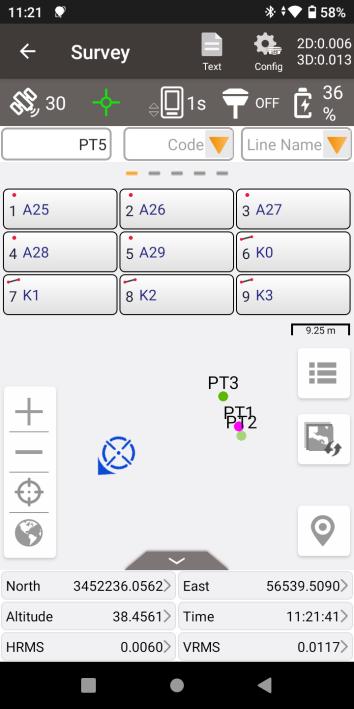
Figure 4.62[]{#_Toc26863 .anchor} Survey Config -- Quick Code
[Stakeout Prompt Tone]: can be enable or disabled.
[Auto Zoom]: When it is turned on, the stakeout graphic interface will be zoomed to the target point and the current position every 3 seconds.
[Stakeout tolerance]: the distance threshold of the stakeout tone. For example, set 0.05 means the stakeout tone beeps every 1 seconds if distance is less than 0.05m.
[Stakeout Prompt Type]: can be North and South direction or Forward and Backward.
[Stakeout Prompt Freq]: can be High or Normal. When selecting High, the stakeout prompt text will be refreshed more frequently than 1Hz.
[Cad Unit]: can be modified to m or mm, for drawings in the CAD Stakeout module.
[Antenna]: Antenna name.
[Type]: height type, can be vertical, slant or pole.
[Ant Height (m)]: value of the antenna height according the specified measuring type.
4.7.2 Display Config
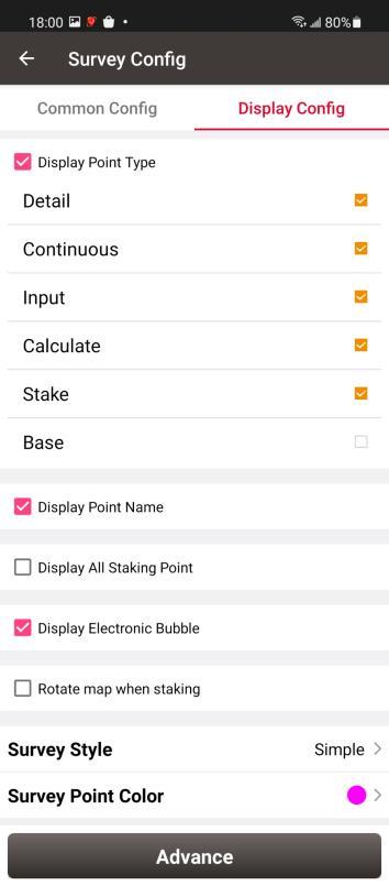
Figure 4.63[]{#_Toc26930 .anchor} Survey Config -- Display Config
Select the Display Point Type, Display Point Name, Display Point Code, Display all staking point, Display Electronic Bubble, Rotate map when staking or Display coordinates when staking according to the application requirement.
Select Survey Style: Simple or Detailed.
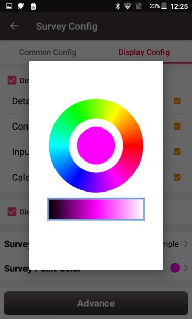
Figure 4.64[]{#_Toc9052 .anchor} Survey Point Color
Click [Survey Point Colour] to select a colour on the outer ring for the survey points and click the inner pie to confirm the colour.

Figure 4.65[]{#_Toc32123 .anchor} Advanced Config for Display Config
Click [Advance] to filter the displayed points.
Base Shift
In 'Auto Start' mode for base station, if the base is moved, re-erected or restarted at an unknown point, base shift should be performed to ensure the points collected by the current base station is consistent with that before the base is moved or powered off. Briefly, find a known point, measure the coordinates of this point, then use this point to calculate the offset of the base shift, apply the base shift to all the survey points under the current base coordinates to make the reference coordinate system of the base remains the same as the previous base station.
The detailed steps are as follows:
Click [Base Shift] to enter the following interface, Figure 4.61 shows the calculation result for the base shift; Figure 4.62 shows the source of the base shift calculation. Click the list icon on the right of GNSS Point to select a survey point which is measured at the known point and click the list icon on the right of Known Point to select a known point in the control point library (details of control point refers to section 2.4 Point). Click [Calculate] and the base shift is calculated automatically. Click [Apply] to apply the base shift to all the points surveyed and to be surveyed under the current base station.
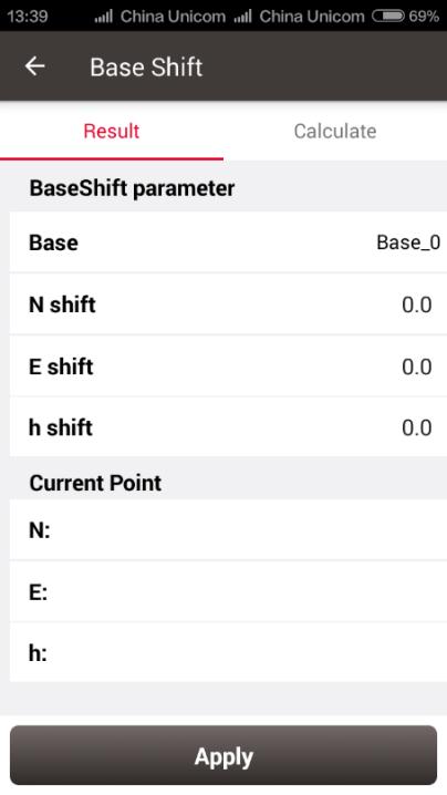
Figure 4.66[]{#_Toc2282 .anchor} Base Shift interface -- 1
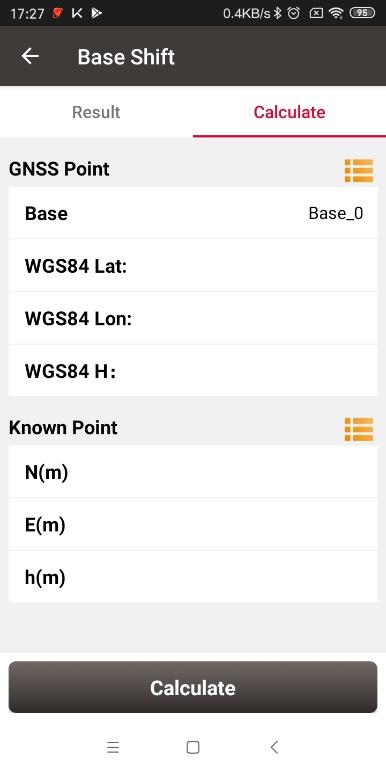
Figure 4.67[]{#_Toc21319 .anchor} Base Shift interface -- 2
At this time, select the base point in the survey point library to view the details. It can be found that the current NEh shift amount is recorded in the base point information, and the NEh coordinates of all the survey points under this base station change accordingly.
If you need to reset (cancel) the base shift, just enter [base shift], and manually modify the three parameters of north shift, east shift and height shift to 0. At this time, return to the survey point library to view the details of the base point. The NEh shift amount in the base point information is automatically changed to 0, and all survey points NEh coordinates under the base station are restored to the coordinates before the base shift.
Road Stakeout
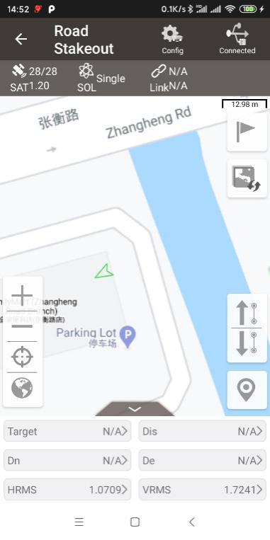
According to the digital designed road created in the road management module, after the software is connected to the high-precision positioning GNSS receiver, enter the road stakeout interface to stake out the designed road stake points and other feature points.
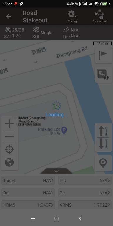
Click [Survey] -> [Road Stakeout], click the  icon to select a road file, the road is drew on the map after the road file is loaded, and then you can start the stakeout. It may take some time for the software to load the newly-built road or modified road for the first time. Once the loading is completed, this road is selected again for stakeout without waiting.
+----------------------------------------------------------------------------------------------------------------------------------------------+----------------------------------------------------------------------------------------------------------------------------------------------+
|  |
|  |
| | |
| Figure 4.68[]{#_Toc29750 .anchor} Road stakeout interface | Figure 4.69[]{#_Toc19676 .anchor} Road data is loading |
+----------------------------------------------------------------------------------------------------------------------------------------------+----------------------------------------------------------------------------------------------------------------------------------------------+
|
| | |
| Figure 4.68[]{#_Toc29750 .anchor} Road stakeout interface | Figure 4.69[]{#_Toc19676 .anchor} Road data is loading |
+----------------------------------------------------------------------------------------------------------------------------------------------+----------------------------------------------------------------------------------------------------------------------------------------------+
Alignment Stakeout
After the loading is completed, select the type as Interval.
It is divided into the options of by interval and by nearby. By interval means starting from the starting mileage point, stake out step by interval according to the set interval. The mileage value of the nearest point on the road to the current position will be obtained after clicking the position icon, so that it is convenient to start the road stakeout from that point immediately. Stakeout by nearby will calculate the nearest point on the road to the current position as the target point at any time, and with the current position moving, the mileage and offset of the corresponding point on the road will change.
Staking to the middle pile, left pile and right pile are allowed in alignment stakeout. The coordinates of the middle pile are calculated according to the alignment and vertical profile, when cross section, super elevation and widening are added to the calculation of the coordinates of the left or right pile.
Then follow the software instructions to move the high-precision GNSS receiver to the design point to complete the stakeout.
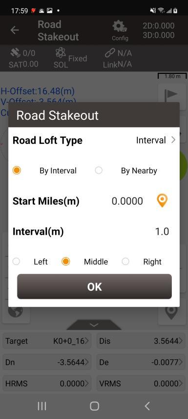
Figure 4.70[]{#_Toc14 .anchor} Road stakeout setting
Cross-section Point Survey
After the loading is completed, select the type as Cross Section (Survey).
The cross-section point survey will start from the cross-section at the starting mileage. When the current mileage cross section point survey is completed, click on the previous or next to jump to another mileage according to the set interval. The mileage value of the nearest point on the road to the current position will be obtained after clicking the position icon, so that it is convenient to start cross-section point survey from the mileage at that point immediately.
In the process of cross-section point survey, the software draws the cross-section at the current mileage and, as the current position moves, the software shows the H-offset, V-offset and Cut or Fill values according to the cross-section.
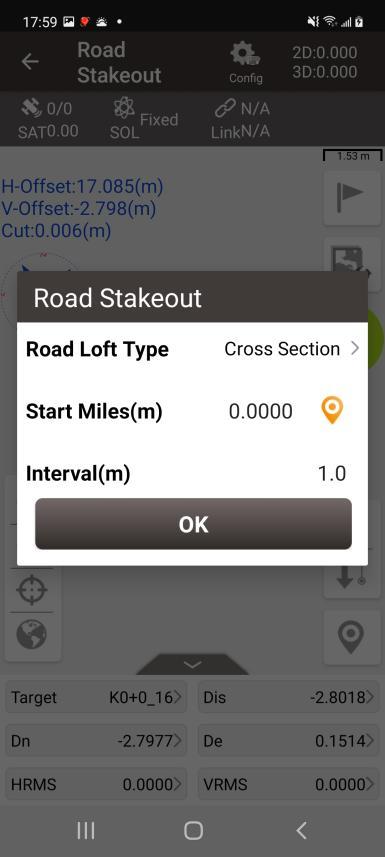
Figure 4.71[]{#_Toc22002 .anchor} Road stakeout setting
Cross-section Point Stakeout
After the loading is completed, select the type as Cross Section (Stake).
The stakeout targets in cross section stakeout are points on the cross section at different mileages in LandXML road. Click on the previous or next to jump to another mileage refers to the LandXML road and click on the left or right to switch the section points at the same mileage.
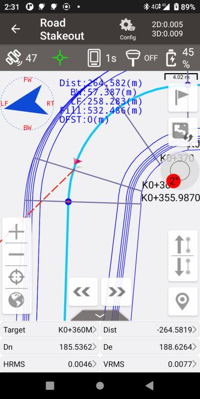
Figure 4.72[]{#_Toc12237 .anchor} Cross Section Stakeout
Surface Stakeout
According to the imported 3dface in DXF files, surface data in LandXML files or created TIN by the custom points selection, when the current position enters within the triangle surface area, the software interpolates the design height of the current position based on the triangle surface data, and indicates the fill or cut value.
The main steps of surface stakeout are as follows:
-
Enter the surface list: click
to enter the surface list after connecting to GNSS receiver.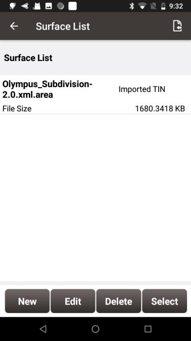
Figure 4.73[]{#_Toc27234 .anchor} Surface List
-
Add stakeout surface: click the icon to select DXF files to import 3dface data or LandXML files to import surface data, or click [New] to select points from the point library to create TIN data.
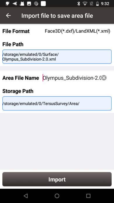
Figure 4.74[]{#_Toc25875 .anchor} Import surface data
-
Edit stakeout surface: select the imported TIN data to edit the offset value, or select the created TIN data to edit the offset value and the points that make up the TIN data.
-
Select the surface to be stakeout: select the surface in the list, and click [Select] to start surface stakeout.
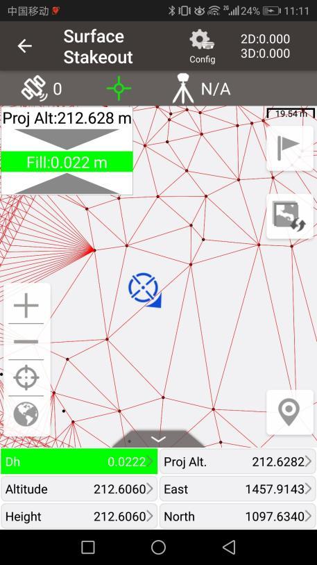
Figure 4.75[]{#_Toc6913 .anchor} Surface stakeout
When the position is within the surface area, the software automatically interpolates the design height value based on the 3dsurface data, and calculates the cut / fill value by subtracting the current height from the design height. When the design height is smaller than the current height, the height deviation is negative and it needs to be cut, the indication is red. When the design height is larger than the current height, the height deviation is positive and it needs to be filled, the indication is blue.
If you need to change the stakeout surface, click the ![]() button and select another surface in the list.
button and select another surface in the list.
CAD Stakeout
CAD stakeout module is used to import CAD files in DXF or DWG format and directly select points and lines on CAD drawings for stakeout.
Click [Survey] -> [CAD Stakeout], select a CAD file in DXF format or DWG format, as shown in the figure below. If there is a recently opened CAD file, it will be displayed in Recent files and can be opened directly by clicking on it.
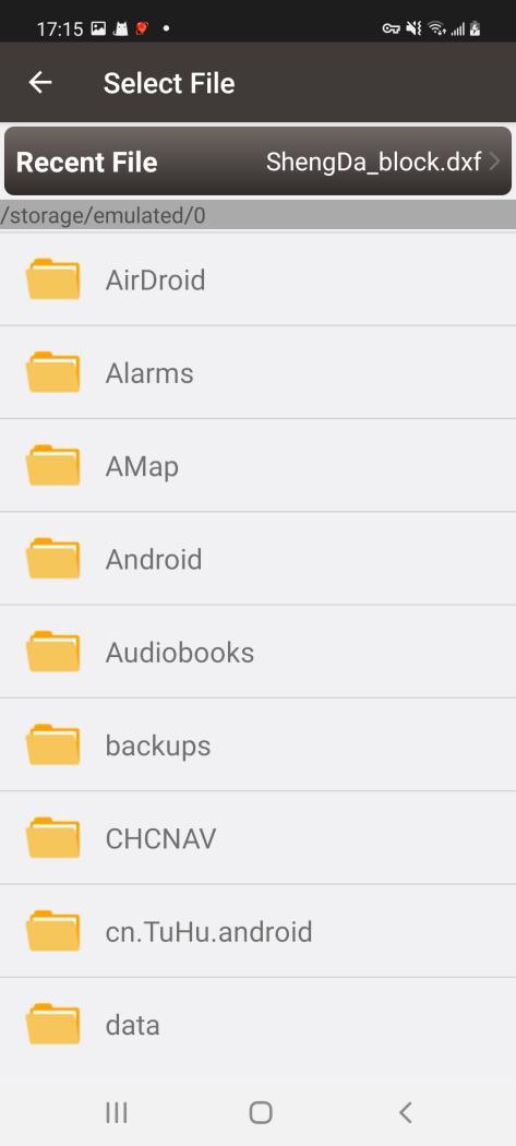
Figure 4.76[]{#_Toc9736 .anchor} Select CAD file
After opening the CAD file, it jumps to the main CAD stakeout interface, the CAD drawing is loaded and displayed, as shown below. Use the point selection tool to select the point on the drawing to stake the point. Click point or line on the drawing directly and then click
  or
or  to stake the point or the line.
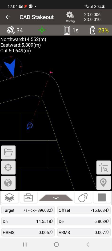
Figure 4.77[]{#_Toc721 .anchor} CAD stakeout
Icon Description
![]() Zoom by current position.
Zoom by current position.
![]() Zoom all.
Zoom all.
Point selection, click on it and the point selection tool will appear on the main screen, press the tool and move to capture the POI, then the point stakeout starts.
![]() Stake point collect, stake the POI and the stakeout ends.
Stake point collect, stake the POI and the stakeout ends.
![]() List button, to display all nodes on the selected line as a list.
List button, to display all nodes on the selected line as a list.
 Layer management, control the display, locking and freezing of different layers.
 Tool set.
 Distance measurement, select two points on the drawing and calculate the distance.
 Area measurement, select points on the drawing and calculate the area and perimeter.
 Find, enter text to search and locate the text.
 Switch the background color, which is currently allowed to be black or white.
 Explode, select a block or polyline and explode it.
 Default state, waiting for the point or line to be selected.
Point stakeout, click the button to start staking the selected point.
Line stakeout, click the button to start staking the selected line.
 Stakeout stop, click it to return to the default state.
In the CAD Stakeout interface,
-
The red flag indicates the location of the stakeout point.
-
The red dotted line is the connection between the current point and the point to be staked.
-
The small blue arrow is the point to be staked.
-
The small blue arrow pointing towards the surveyor heading.
-
The big blue arrow prompts the surveyor that the point to be staked is in the front/rear/left/right position.
-
The blue number shows the distance from the point to be staked in different directions.
CAD Survey
CAD stakeout module is used to import CAD files in DXF or DWG format and use the CAD drawings as a reference map for points survey.
In CAD Survey, select a CAD file in DXF or DWG format, open the file and successfully load the CAD drawing as shown below. Click the Survey button to start point survey.
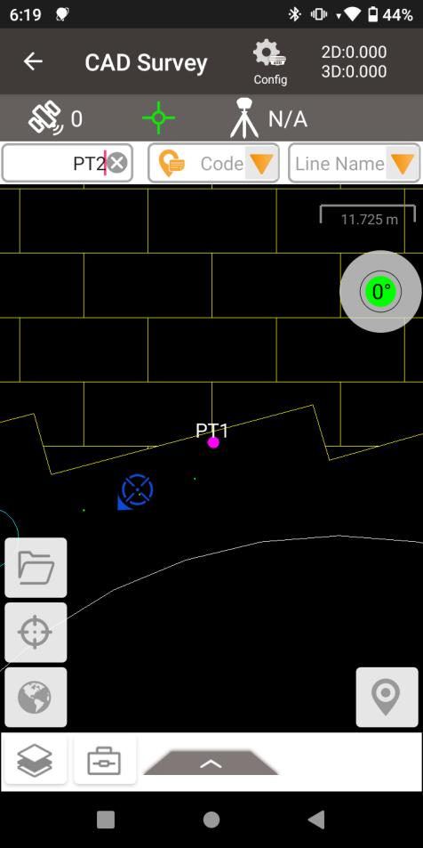
Figure 4.78[]{#_Toc26199 .anchor} CAD survey
Icon Description
![]() Zoom by current position.
Zoom by current position.
![]() Zoom all.
Zoom all.
![]() Click to start point survey.
Click to start point survey.
Layer management, control the display, locking and freezing of different layers.
Tool set.
Distance measurement, select two points on the drawing and calculate the distance.
Area measurement, select points on the drawing and calculate the area and perimeter.
Find, enter text to search and locate the text.
Switch the background color, which is currently allowed to be black or white.
Visual Positioning
Visual Positioning is available for Oscar Trek and TS21, where the measurement results of the target points are obtained by taking a video and getting the coordinates of the points directly on photos.
4.13.1 Take Video
Turn on Tilt first, input the correct pole height and finish the tilt initialization. Go to [Survey] - [Visual Positioning]. The main interface shows visual camera shooting screen. When the upper-right precision estimate is too large and the icon shows red, shake the pole or move the device according to the animation shown to take tilt initialization and visual positioning initialization until the upper-right precision estimate meets the requirements, the icon shows green and the animation disappears.
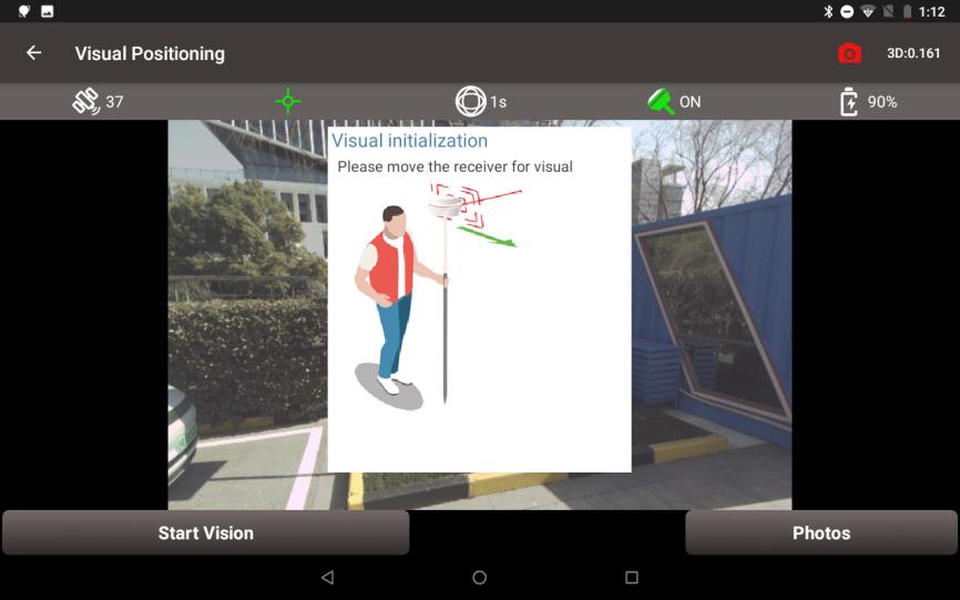
Figure 4.79[]{#_Toc14467 .anchor} Visual Positioning Initialization
Click [Start Vision], keep the visual camera facing the target points, move the device to take photos of the target points from different directions. Click [Stop] to end recording. Check the quality and the number of pictures for this visual positioning and enter the group name.
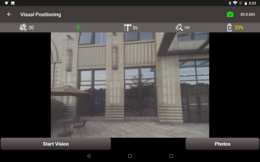
Figure 4.80[]{#_Toc9430 .anchor} Visual Positioning Start
Note:
-
Ensure that the device is located in an open sky environment, without any obstruction to the GNSS antenna, throughout the initialization process.
-
Remember not to rotate the receiver violently during the initialization process. To improve visual measurement performance, focus on ensuring sufficient moving, as rotation does not enhance it.
-
During the initialization phase, the camera should be turned back toward the surveyor to avoid obstruction of the view by their body.
-
In the moving stage, the camera should not be pointed at non-textured objects, such as the sky and white walls.
3D values in the upper right corner indicates the predicted 3D measuring error at 10 meter distance.
4.13.2 Photo Groups
Click [Photos] to view all groups of photos taken for further measurement. Click on the mode button on the upper right corner in photos screen, there are four modes to take measurement for visual positioning.
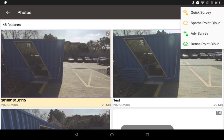
Figure 4.81[]{#_Toc31034 .anchor} Four Measurement Modes
If needed, click the [Multi-select] button and choose the photo group to export. Then connect the Oscar Trek or TS21 to a computer and locate the exported image group in the directory for 3D modeling post-processing
4.13.3 Quick Survey
This section introduces Quick Survey mode. Quick Survey use the traditional Pick point - Calculate - Adjust process. Calculations are performed at the receiver side. The advantage of quick survey is that there are no controller performance requirements and calculations are faster.
1) Click on a photo group to slide through all the photos in the group.
2) Click on one of the photos that contains target points to enter the photo measurement interface. Click the target point directly on the picture, then the clicked position will show a blue cross, and you can change the position of the blue cross by dragging. You can also zoom in and out of the picture to make it easier to align the blue cross to the target point.
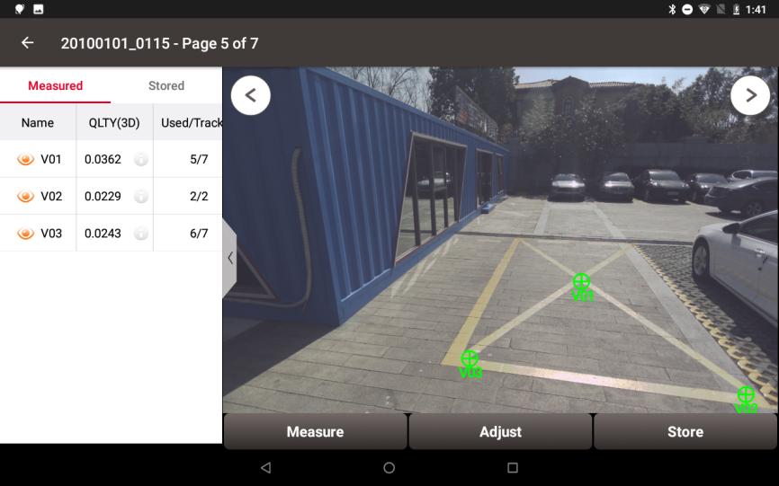
Figure 4.82[]{#_Toc3177 .anchor} Quick Survey
3) Click [Measure], the blue cross will turn green, and the measured point list will show 3D quality and the number of used photos. Continue to select other target points in this way.
4) Switch to other photos, check whether the green cross is aligned with the target point. If failed to match on some photos, it will be shown as a red circle.
5) Click [Adjust], select the point and drag to align target manually. It will be recalculated and generally the quality will become higher and the used photos will increase.
6) Confirm that all points are measured correctly. Click the white icon ![]() to check the detailed information and edit point name. Then click [Store] and enter points information to store visual positioning points into the point database.
to check the detailed information and edit point name. Then click [Store] and enter points information to store visual positioning points into the point database.
Note:
-
Hold the receiver steady and keep a normal walking speed while capturing images.
-
For optimal accuracy and performance, capture the object of interest from a distance between 2m and 10m.
-
Avoid using it in dark conditions or when directly facing the sun, as it may lead to difficulty in recognizing enough features in the captured images to make a match.
-
Try to select feature points on an image directly in front of the target object. For example, choose an image in the middle of the captured images.
-
Multiple feature points can be selected at a time.
4.13.4 Sparse Point Cloud
This section introduces Sparse Point Cloud mode. In this mode, you need to circle the position around the target point first, then after the sparse point cloud being generated, select the nearest point in the sparse point cloud to obtain coordinates directly.
Calculations are performed at the receiver side. The advantage of this mode is that there are no controller performance requirements and calculations are faster, while at the same time the operations are simpler without adjustments.
1) Click on a photo group and click on one of the photos that contains target points. Click the circle button ![]() and draw a circle containing the target point.
and draw a circle containing the target point.
2) After the calculation, the sparse point cloud of the circled position will be displayed on the picture. If the points in the sparse point cloud are too far away from the target, draw another circle near the target position to generate more point clouds.
3) Click the select button  and click one of the point in sparse point cloud to select. If a wrong point is selected, use the button to cancel the selection.
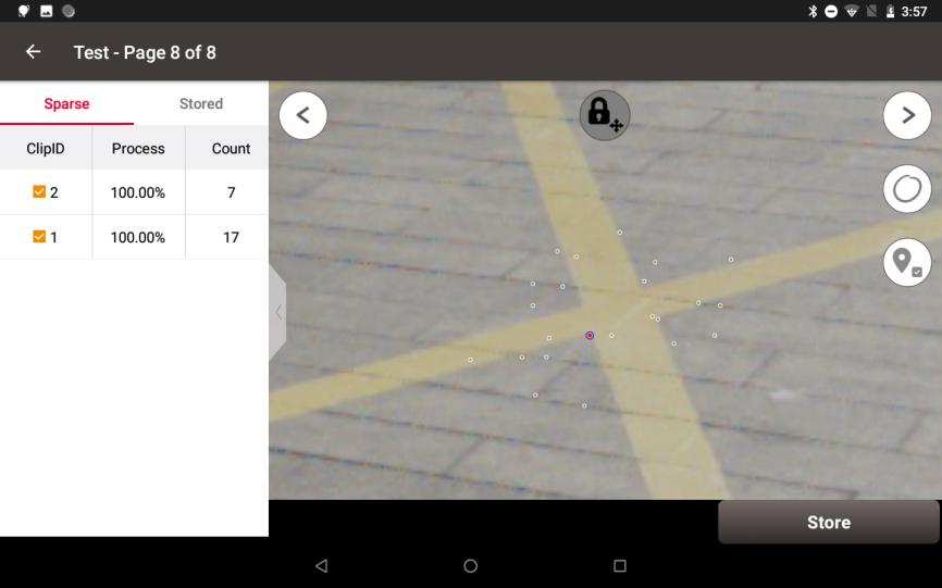
Figure 4.83[]{#_Toc28818 .anchor} Sparse Point Cloud
4) Continue to select other target points in the way above. Then click [Store] and enter points information to store visual positioning points into the point database.
4.13.5 Adv Survey
This section introduces Adv Survey mode. In Advanced Survey mode, the software will prepare the dense point cloud automatically first. The user only need to pick the point on the picture and the software will automatically generate the dense point cloud around the target, select the corresponding point in point cloud and give the results directly.
Calculations are performed at the controller side and therefore has performance requirements for the controller. The advantage of this mode is that the point cloud is dense and accurate, simplest for the user to operate and very accurate in measurement.
1) Click on a photo group and click on one of the photos that contains target points. It may take some time to prepare dense point cloud.
2) Click the target point directly on the picture, then the clicked position will show a blue cross, and you can change the position of the blue cross by dragging. You can also zoom in and out of the picture to make it easier to align the blue cross to the target point.
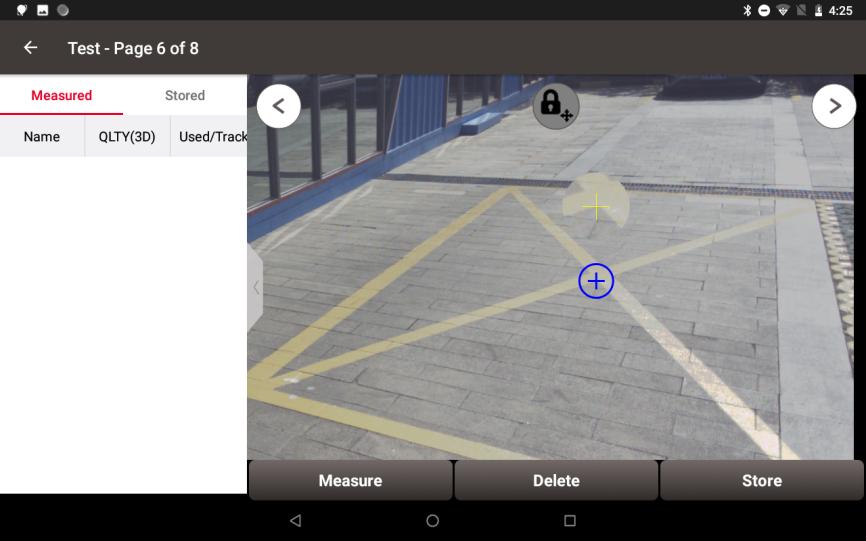
Figure 4.84[]{#_Toc7204 .anchor} Advanced Survey
3) Click [Measure], and it may take some time to calculate the dense point cloud. The blue cross will turn green after the calculation. Select other target points in the same way.
4) Click the white icon ![]() to check the detailed information and edit point name. Click [Store] to store visual positioning points into the point database.
to check the detailed information and edit point name. Click [Store] to store visual positioning points into the point database.
4.13.6 Dense Point Cloud
This section introduces Dense Point Cloud mode. The measurement process in this mode is similar to that of the sparse point cloud. More importantly, we can export the dense point cloud.
Calculations are performed at the controller side and therefore has performance requirements for the controller.
-
Click on a photo group and click on one of the photos that contains target points. It may take some time to prepare dense point cloud.
2) Click the button
 and wait for global 3D point cloud reconstruction results the dense point cloud of the circled position will be displayed on the picture.
3) Click [Export] and select the path to the las file. Then open las file to check the dense point cloud generated by Oscar Trek or TS21 visual positioning on site.
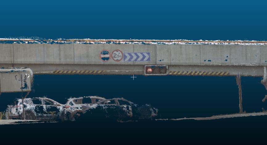
Figure 4.85[]{#_Toc16865 .anchor} Export Dense Point Clouds