Project
-
Project
-
CRS (CooRdinate System)
-
Code
-
Point
-
Line
-
Road
-
Import
-
Export
-
Settings
-
Cloud Setting
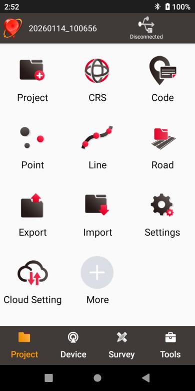
Figure 2.1[]{#_Toc9283 .anchor} Functions under Project
Project
This section introduces how to create a new project, open / delete / edit an existing project.
New
A new project is necessary to manage all the data. On the Nuwa main interface as shown in Figure 1.10, click [Project] - > [New] to go to the following interface.
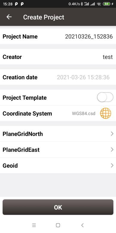
Figure 2.2[]{#_Toc26248 .anchor} Create Project interface
[Project Name]: input the project name
[Creator]: input the name of the operator
[Creation date]: the date and time generates automatically.
[Project Template]: use an existing project settings
[Coordinate System]/ [Source Project]: select a coordinate system if project template is not turned on; select a source project if using a project template.
[PlaneGridNorth]: select plane grid in the list, or click More to download more grid file online.
[PlaneGridEast]: select plane grid in the list, or click More to download more grid file online.
[Geoid]: select geoid model in the list, or click More to download more geoid file online.
Note: (1) If the grid file or geoid file is already selected in the parameters of the selected coordinate system, the selected grid file or geoid file will be automatically filled in below when the new project is created.
(2) If the grid file or geoid file is selected here, they will be applied to this project after new project is successfully created.
(3) If the grid file or geoid file is selected here, but the file is actually not available in the controller InternalStorage\TersusSurvey related path, then it will automatically jump to the download interface to search and download the file. Only when the selected grid file or geoid file is downloaded, or when the file is deselected, can the project continue to be created.
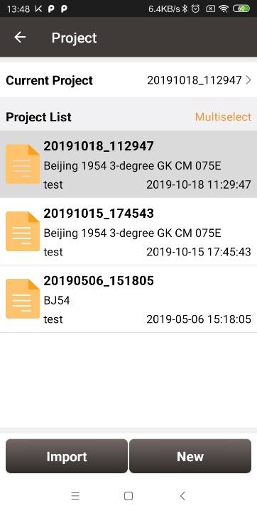
Figure 2.3[]{#_Toc23457 .anchor} New project created
After a project is created, it will prompt out a window asking whether close the current project and open the newly created project. The projects in the list are sorted in reverse chronological order. Refer to section 2.1.5 for more details about project property.
Import
In the Figure 2.3, an existing project can be imported from the storage of the android device by clicking [Import] on the bottom left of the interface.
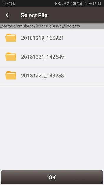
Figure 2.4[]{#_Toc26685 .anchor} Project folders in an Android device
When importing projects from other sources, click [Import], select the Project folder under TersusSurvey which is shown in Figure 2.4, and click [OK] and Nuwa imports all the projects in this folder.
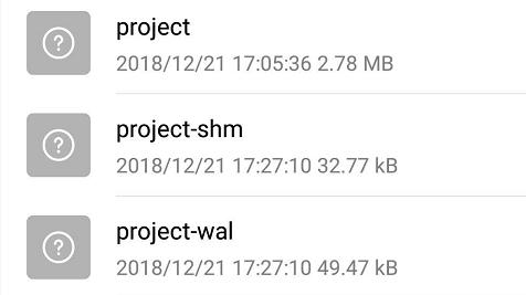
Figure 2.5[]{#_Toc19158 .anchor} Sketch file containing the project info
Note: The imported project file should have a sketch file containing the project information (Project / Project-shm / Project-wal).
Open
If there is need to operate in an existing project, find it in the project list and click it. Nuwa prompts to open the project, click [OK].
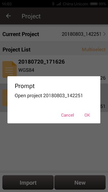
Figure 2.6[]{#_Toc11429 .anchor} Open an existing project
Delete
Click [Multiselect] at the right side of Project List, select (single select, inverse select or select all) projects to be deleted. After the projects are selected, click [Delete] button to delete them. Nuwa prompts to confirm, click [OK] to complete the deletion.
Note: The current Project cannot be deleted in Nuwa app.
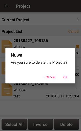
Figure 2.7[]{#_Toc20290 .anchor} Delete Project
Edit Project Property
If a project is opened, the coordinate system can be edited, including ellipsoid, projection method and coordination transformation.
Figure 2.8[]{#_Toc25648 .anchor} Project List
Click the [Current Project] to enter Project Property interface.
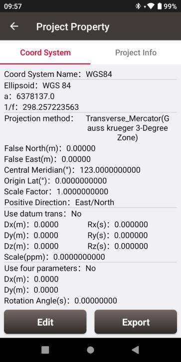
Figure 2.9[]{#_Toc17896 .anchor} Project Property
Click [Edit] to input the ellipsoid parameters, projection type and coordination transformation, refer to section 2.2.1 for details. Click [Export] to save the coordinate system and parameters of the current project as a new coordinate system csd file for sharing or use in other projects.
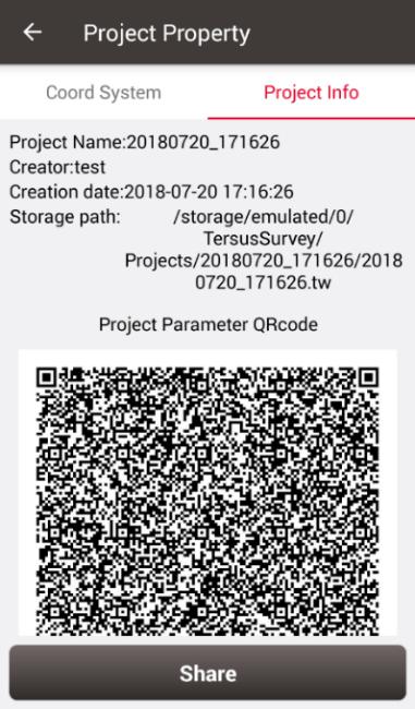
Figure 2.10[]{#_Toc17955 .anchor} Share Project Info
Click [Share] to share the project parameters with others. The detailed usage refers to section 2.2.1.
CRS (CooRdinate System)
Nuwa app supports user-defined coordinate system. A user-defined coordinate system can be saved as a template. A CRS can be created, imported, edited and deleted in the CRS management interface.
On the Nuwa main interface as shown in Figure 1.10, click [CRS] to get the coordinate system list which is shown below.
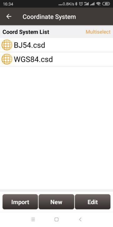 Figure 2.11[]{#_Toc9063 .anchor} Coordinate System List
New CRS
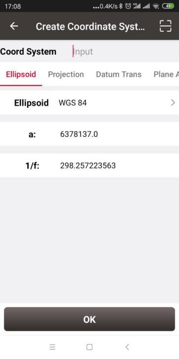
Figure 2.12[]{#_Toc2098 .anchor} Create a new CRS
Click [New] to create a new CRS, input the coordinate system name, select the right ellipsoid, projection, datum transformation, plane adjustment, and height fitting as per the following screenshots:
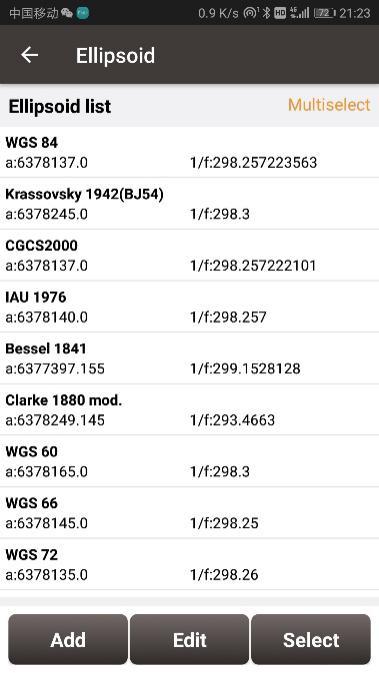
Figure 2.13[]{#_Toc18477 .anchor} Ellipsoid list
[Ellipsoid]: Select the correct ellipsoid parameters, including ellipsoid name, semi-major axis, inverse flattening, etc. For a predefined ellipsoid, it automatically fills the semi-major axis and inverse flattening after selecting the ellipsoid; if the ellipsoid that meets the requirements is not found in the predefined ellipsoid, and you have the parameters of the ellipsoid, you can [Add] an ellipsoid to the list, enter your parameters and select it; If the ellipsoid that meets the requirements is not found in the predefined ellipsoid and you do not have the parameters for this ellipsoid, please contact Tersus technical support.
Note: The default ellipsoid is WGS84.
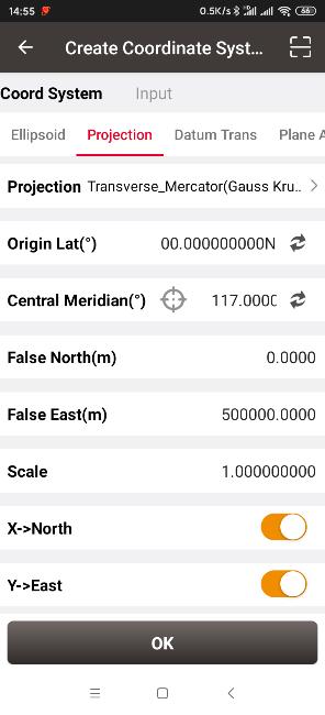
Figure 2.14[]{#_Toc29776 .anchor} Projection interface
[Projection]: Including Transverse Mercator, UTM, Lambert conformal conic 1SP, Lambert conformal conic 2SP, and etc. When a receiver is connected with Nuwa, click the icon ![]() to round the current longitude as the central meridian. The projection is listed as below, if the required projection is not found in the predefined projection list, please contact Tersus technical support.
to round the current longitude as the central meridian. The projection is listed as below, if the required projection is not found in the predefined projection list, please contact Tersus technical support.
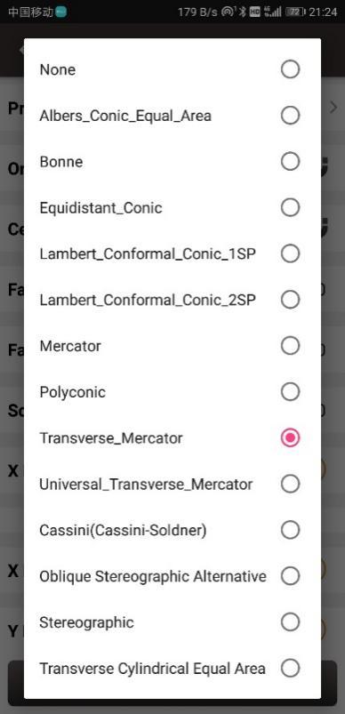
Figure 2.15[]{#_Toc25831 .anchor} Projection list
Origin latitude, central meridian and other parameters can also be configured in Projection interface which is shown above. Fill in these information according to the actual needs. Turn on [X->North] to indicate that the positive part of X axis is north, negative part is south. Turn on [Y->East] to indicate that the positive part of Y axis is east, negative part is west.
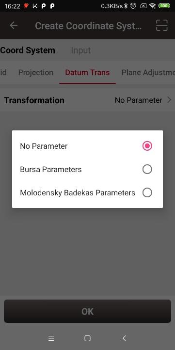
Figure 2.16[]{#_Toc4294 .anchor} Datum transformation options
[Datum Transformation]: Datum transformation is necessary when the source ellipsoid is different from the target ellipsoid. There are three options: No parameter, Bursa Parameters and Molodensky Badekas Parameters.
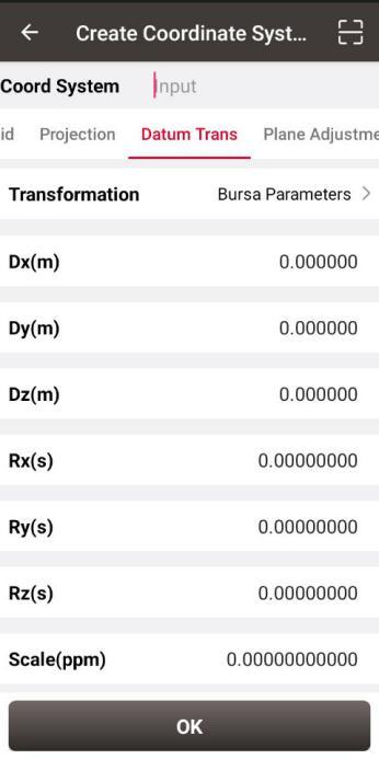
Figure 2.17[]{#_Toc827 .anchor} Bursa Parameters
[Bursa Parameter]: Axis shift, rotation and scale would be introduced in the datum transformation. Bursa-Wolf seven-parameter model is used from local coordinate to WGS84 system. At least three known points are necessary for accurate transformation. Only X/Y/Z shifts are required only if three parameter transformation is needed.
+---------------------------------------------------------------------------------------------------------------------------------------------+---------------------------------------------------------------------------------------------------------------------------------------------+
|  |
|  |
| | |
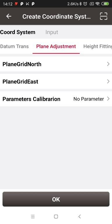
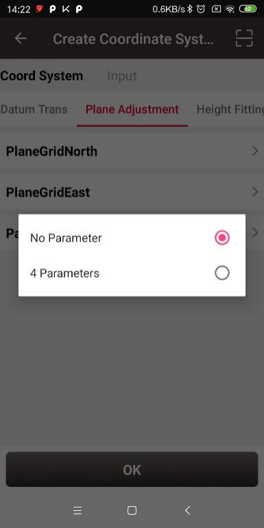
| Figure 2.18[]{#_Toc3714 .anchor} Plane adjustment interface | Figure 2.19[]{#_Toc1722 .anchor} Plane adjustment options |
+---------------------------------------------------------------------------------------------------------------------------------------------+---------------------------------------------------------------------------------------------------------------------------------------------+
|
| | |
| Figure 2.18[]{#_Toc3714 .anchor} Plane adjustment interface | Figure 2.19[]{#_Toc1722 .anchor} Plane adjustment options |
+---------------------------------------------------------------------------------------------------------------------------------------------+---------------------------------------------------------------------------------------------------------------------------------------------+
[Plane Adjustment]: Plane adjustment is for the transformation between two planes. There are two options for parameters calibration: No parameter and 4 parameters. The detailed information and usage of plane grid refer to section 2.2.5.
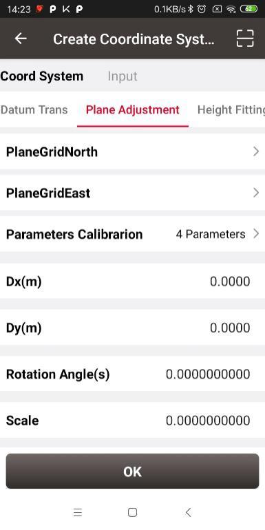
Figure 2.20[]{#_Toc29106 .anchor} 4 Parameters
[4 Parameters]: X/Y axis shift, rotation angle and scale are necessary to be input as above. These parameters can be calculated from site calibration, details refer to section 4.5.1.
+---------------------------------------------------------------------------------------------------------------------------------------------+---------------------------------------------------------------------------------------------------------------------------------------------+
|  |
|  |
| | |
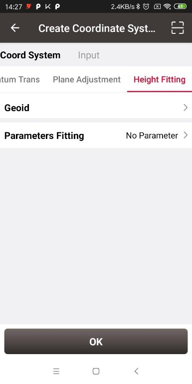
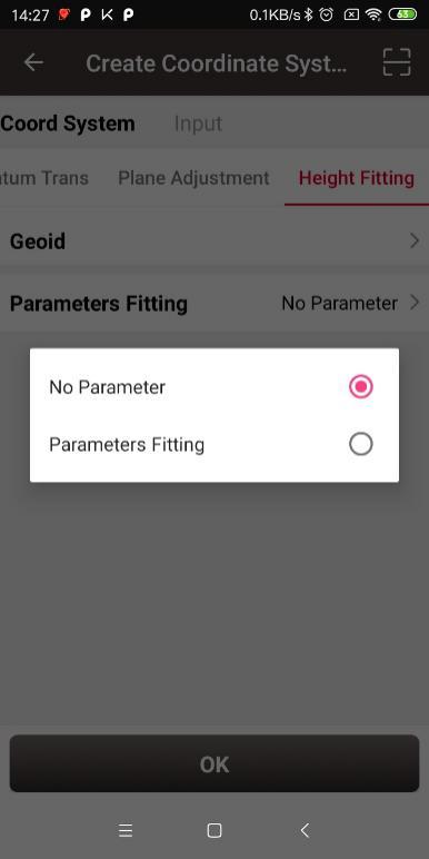
| Figure 2.21[]{#_Toc14864 .anchor} Height fitting interface | Figure 2.22[]{#_Toc10386 .anchor} Parameters fitting options |
+---------------------------------------------------------------------------------------------------------------------------------------------+---------------------------------------------------------------------------------------------------------------------------------------------+
|
| | |
| Figure 2.21[]{#_Toc14864 .anchor} Height fitting interface | Figure 2.22[]{#_Toc10386 .anchor} Parameters fitting options |
+---------------------------------------------------------------------------------------------------------------------------------------------+---------------------------------------------------------------------------------------------------------------------------------------------+
[Height Fitting]: Height fitting has two options: Geoid and Parameters Fitting. Parameters fitting includes no parameter and detailed parameters fitting.
[Geoid]: Geoid supports ggf, grd, gsf, osgb, mnt and isg format files, the detailed information and usage of geoid files refer to section 2.2.5.
[Parameters Fitting]: Currently three algorithms are supported: fixed difference correction, plane fitting and surface fitting. The parameters needed can be calculated from site calibration, details refer to section 4.5.2.
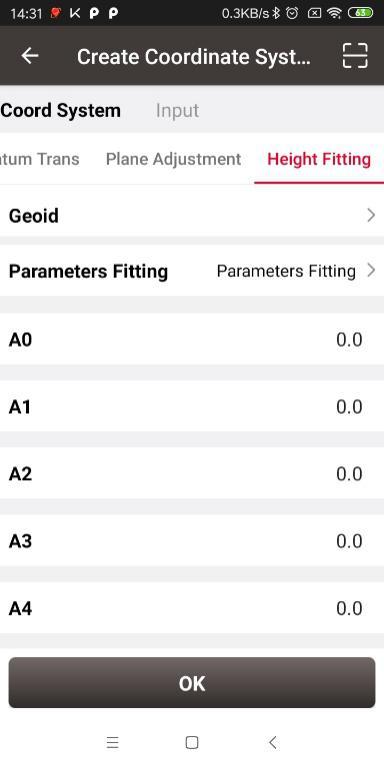
Figure 2.23[]{#_Toc10305 .anchor} Height Fitting -- Parameters Fitting
[TAP Fitting]: When working with TAP mode, if may be necessary to perform frame and epoch conversion calculations for the PPP results. Select the target frame and epoch here, and then manually input or use the predefined velocity field data for the conversion.
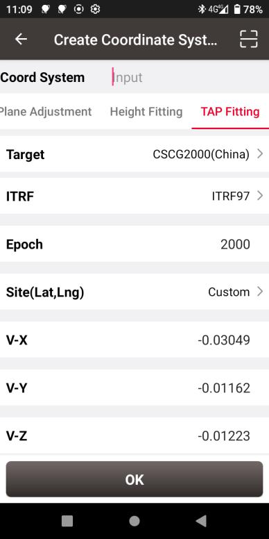
Figure 2.24[]{#_Toc23956 .anchor} TAP Fitting
After setting all parameters to create a new coordinate system, click [OK] to complete the configuration.
Click the scan icon ![]() in the top right corner of Figure 2.12, open the camera to scan other surveyor's coordinate system parameters QR code to copy information for creating a new CRS.
in the top right corner of Figure 2.12, open the camera to scan other surveyor's coordinate system parameters QR code to copy information for creating a new CRS.
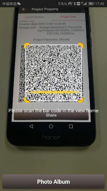
Figure 2.25[]{#_Toc19989 .anchor} Scan QR code to get CRS info
The following shows detailed steps:
-
The copied surveyor opens in turn: [Project] -> [Current Project] -> [Project Information], then displays the complete QR code;
-
The current surveyor opens the camera when creating new CRS to scan the QR code displayed as shown in Figure 2.24 above and can copy its coordinate system parameters. The QR code screenshot in photo album can also be scanned to obtain the CRS parameters.
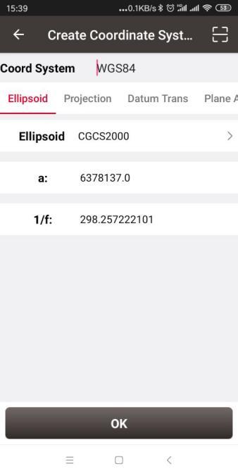
Figure 2.26[]{#_Toc22086 .anchor} CRS info obtained by scanning QR code
- The coordinate system parameters are obtained as shown in the figure above.
Import CRS
Click [Import] on the bottom left of CRS interface which is shown in Figure 2.11, it shows predefined coordinate systems for users to choose.
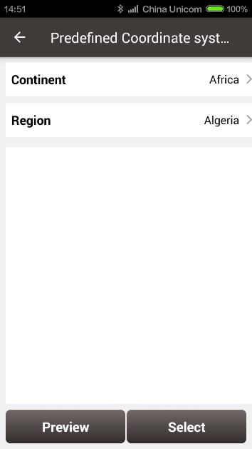
Figure 2.27[]{#_Toc17293 .anchor} Predefined CRS
In the figure above, the predefined coordinate systems are classified by continent and region.
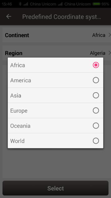
Figure 2.28[]{#_Toc24918 .anchor} Continent options
The continent option includes Africa, America, Asia, Europe, Oceania and World as shown in the figure above. Select a continent, a country or a region, then select a CRS and click [Preview].
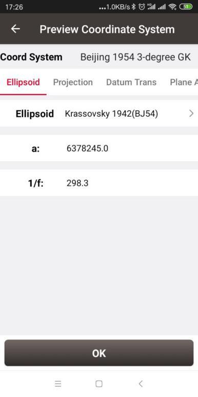
Figure 2.29[]{#_Toc8302 .anchor} Preview of predefined CRS
The above figure is a preview of 'Beijing 1954 3-degree GK CM 075E' coordinate system. Click [OK] and [Select] this CRS, the CRS file is imported to Coordinate System List as shown in the figure below.
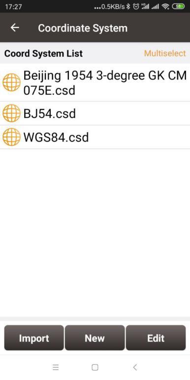
Figure 2.30[]{#_Toc12866 .anchor} Example of CRS import
If the user cannot find the coordinate system of their country or region, but has ellipsoid, projection, datum transformation and other related parameters, you can create a new coordinate system or contact Tersus technical support and we help you create one.
Edit CRS
Click an existing CRS and click [Edit] to enter the Edit Coordinate System interface, refer to the following screenshot:
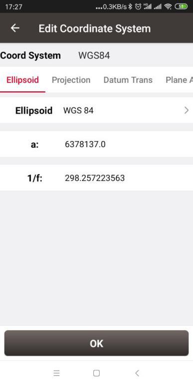
Figure 2.31[]{#_Toc32469 .anchor} Edit Coordinate System
Delete CRS
The default two CRS cannot be deleted. Click [Multiselect] to select the CRS to be deleted and click [Delete] to finish the deletion.
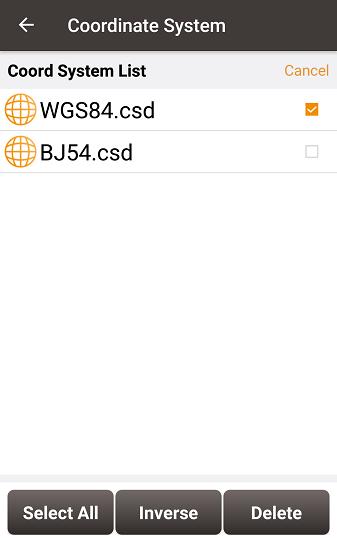
Figure 2.32[]{#_Toc21422 .anchor} Delete CRS
Plane Grid and Geoid
Plane Grid and Geoid are adjustment methods for plane and height, which can improve survey accuracy.
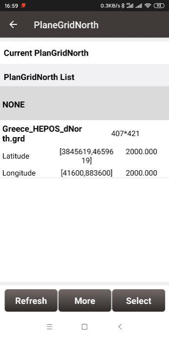
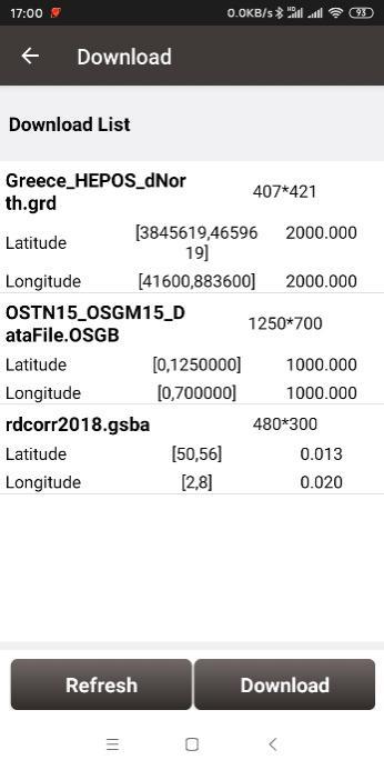
Plane Grid includes plane grid north and plane grid east. Click [PlaneGridNorth] in Figure 2.18 Plane adjustment interface, it enters plane grid north list shown as below. Click [More] to enter download list, the plane grid files can be downloaded from online server. Click [Refresh] to view the current available plane grid files. The plane grid file supports .ggf, .grd, .gsf, and .osgb format. If customer cannot find suitable plane grid file, feel free to contact Tersus support via email support@tersus-gnss.com .
+---------------------------------------------------------------------------------------------------------------------------------------------+---------------------------------------------------------------------------------------------------------------------------------------------+
|  |
|  |
| | |
| Figure 2.33[]{#_Toc23322 .anchor} Plane Grid list | Figure 2.34[]{#_Toc9828 .anchor} Plane Grid download list |
+---------------------------------------------------------------------------------------------------------------------------------------------+---------------------------------------------------------------------------------------------------------------------------------------------+
|
| | |
| Figure 2.33[]{#_Toc23322 .anchor} Plane Grid list | Figure 2.34[]{#_Toc9828 .anchor} Plane Grid download list |
+---------------------------------------------------------------------------------------------------------------------------------------------+---------------------------------------------------------------------------------------------------------------------------------------------+
After downloading a required plane grid file, select it in the plane grid list and it returns to the plane adjustment interface.
Setting the PlaneGridEast is the same with the above method of setting PlaneGridNorth.
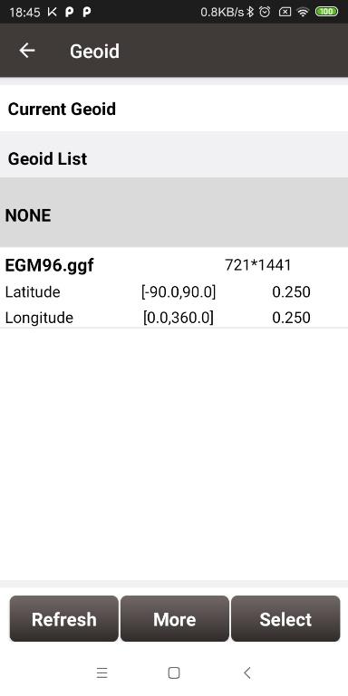
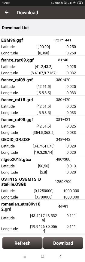
Geoid supports ggf, grd, gsf, osgb, mnt and isg format files, it optimizes data loading, reduces waiting time for different devices, simplifies algorithm calculation process and saves system resources. In a CRS setting, click [Geoid] under Height Fitting tab enter Geoid list which is shown as below. The list shows the coverage latitude, longitude and resolution of the corresponding geoid model. Click [More] to enter download list, the geoid files can be downloaded from online server.
+---------------------------------------------------------------------------------------------------------------------------------------------+--------------------------------------------------------------------------------------------------------------------------------------------+
|  |
|  |
| | |
| Figure 2.35[]{#_Toc11001 .anchor} Geoid list | Figure 2.36[]{#_Toc21364 .anchor} Geoid download list |
+---------------------------------------------------------------------------------------------------------------------------------------------+--------------------------------------------------------------------------------------------------------------------------------------------+
|
| | |
| Figure 2.35[]{#_Toc11001 .anchor} Geoid list | Figure 2.36[]{#_Toc21364 .anchor} Geoid download list |
+---------------------------------------------------------------------------------------------------------------------------------------------+--------------------------------------------------------------------------------------------------------------------------------------------+
Click [Refresh] to view the current available geoid files. Contact Tersus Technical Support support@tersus-gnss.com to inquire more if customer cannot find suitable Geoid files. After downloading a required geoid file, select it in the geoid list and it returns to the height fitting interface.
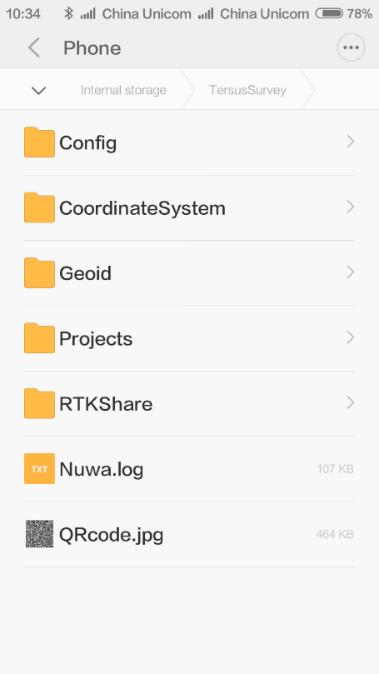
Figure 2.37[]{#_Toc3697 .anchor} Explore Geoid folder in the android device
Another method of importing geoid files: manually copy and paste the Geoid files under the Geoid folder of TersusSurvey as shown above, back to the Geoid list interface and click [Refresh] to view the available Geoid list as shown below.
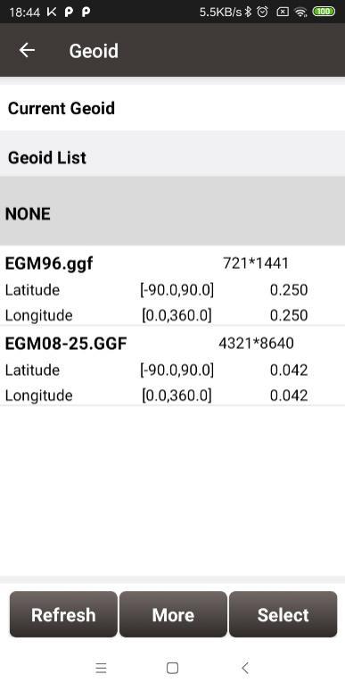
Figure 2.38[]{#_Toc17849 .anchor} Refresh to view the Geoid list
Select one suitable Geoid model and click [Select] to complete the Geoid configuration, and it returns to the height fitting interface.
Code
Nuwa now supports selecting code or entering code, and switch to survey a point feature or a line feature according to the type of the code. Here in the code module, manage the code of the current project.
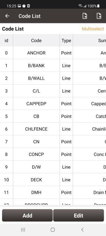
Figure 2.39[]{#_Toc5956 .anchor} Code List
-
Add Code
Click the Add button, then enter the interface as below.
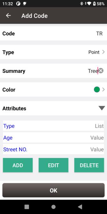
Figure 2.40[]{#_Toc12688 .anchor} Add Code
Input the code to be added, select the type of the code as Point or Line, input the summary of the code, and select color for features with this code. Set attributes of the code if needed, click to add or edit the list type attribute fields and the value type attribute fields. You will be able to enter the attributes based on preset fields in point measurement or point editing.
-
Edit Code
Select a code in the code list, click the Edit button, then enter the Edit Code interface.
Edit the code, the type of the code, the summary or the attributes, then click OK to Edit the code.
-
Delete Code
Click Multiselect, then select the codes to be delete in the code list, click Delete to delete the codes.
-
Import and Export Code
Click the Import button on the upper left to import codes to the current code list. Click the Export button on the upper right to export all the codes in the current code list.
Point
Point library includes survey point library, control point library and staking point library.
It is also supported for a project to contain multiple point library database files.
2.4.1 Survey Point
Click [Project] -> [Point] and see the survey point library as below.
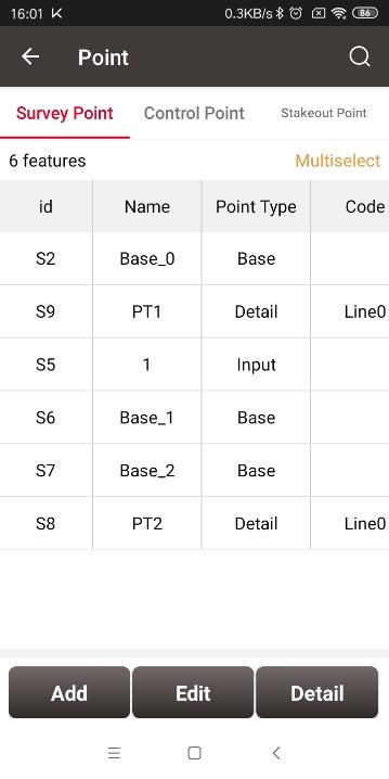
Figure 2.41[]{#_Toc32401 .anchor} Survey Point Interface
In the survey point library interface, slide in the left or right direction to check the point information, such as coordinates, collection time, and etc. Click on the table header to sort the points in the list.
- Add survey point
Under the Survey Point interface, click [Add] to enter the Add Point interface.
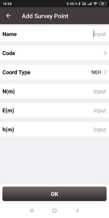 Figure 2.42[]{#_Toc23260 .anchor} Add Survey Point
Fill in the point name and code, choose the coordinate type (including two types: BLH and NEH), fill in the coordinate values, click [OK] to add a new survey point. The point type of the added survey point is called Input Point.
- Edit survey point
In the survey point interface, choose a points to be edited, and click [Edit] to enter the Edit interface.
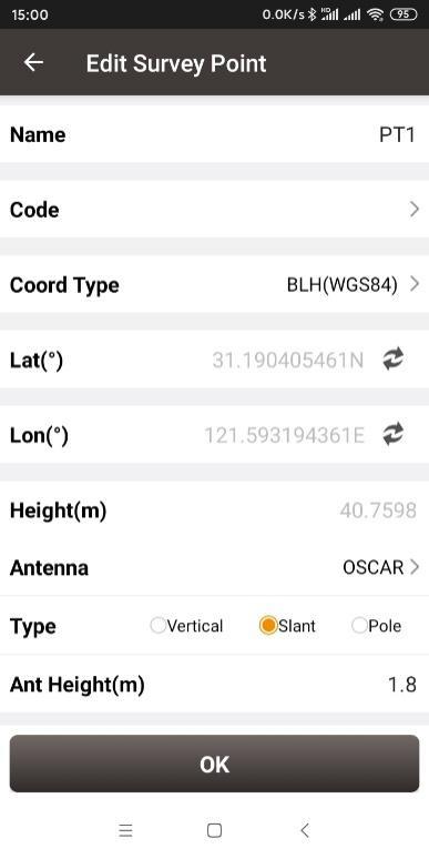 Figure 2.43[]{#_Toc25456 .anchor} Edit Survey Point
Note: The base point and calculated point cannot be edited; all info of the input point can be edited; only antenna info of the detailed point, continuous point and stake point can be edited.
- View details of survey point
In the survey point interface, choose a point and click [Detail] to view details of this point.
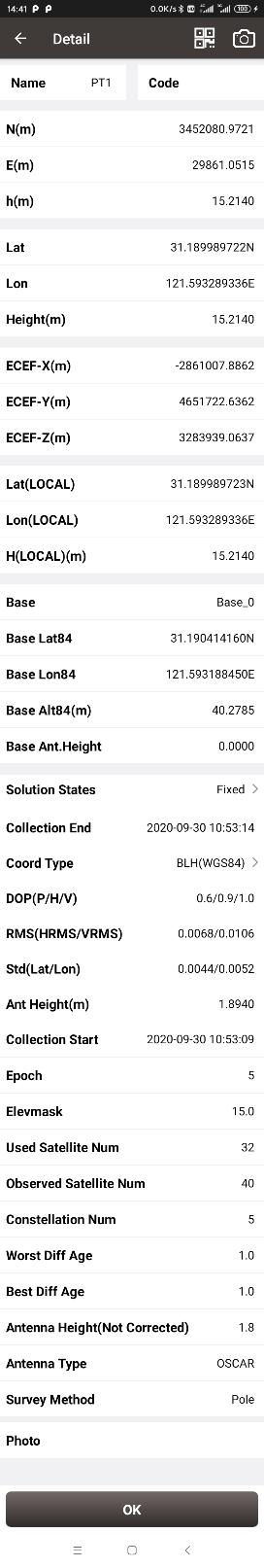 Figure 2.44[]{#_Toc30349 .anchor} View details of Survey Point
On the upper right corner there are two icons: QR code icon ![]() and camera icon
and camera icon ![]() . The detailed descriptions are as below.
. The detailed descriptions are as below.
a. Share the point via QR code. Click ![]() icon to generate the QR code of this survey point. This QR codes contains the point name, code and coordinate information separated by a comma. Other surveyor can obtain these information by scanning this QR code.
icon to generate the QR code of this survey point. This QR codes contains the point name, code and coordinate information separated by a comma. Other surveyor can obtain these information by scanning this QR code.
b. Photo of the survey point. Click ![]() to take a photo using system camera. The photo will be displayed at the bottom of the point detail for preview. The photo is named with point name plus shooting time. The photos are stored under the folder of TersusSurvey/Projects/ProjectName.
to take a photo using system camera. The photo will be displayed at the bottom of the point detail for preview. The photo is named with point name plus shooting time. The photos are stored under the folder of TersusSurvey/Projects/ProjectName.
<!-- -->
- Graphic display
In the survey point interface, click the up-right
icon to enter graphic interface.
In graphic interface, zooming, panning and online maps are supported.
In graphic interface, the selection of points is supported. For example, in some tools, click the point selection button and enter the point library, then click the graphic display button and enter the graphic interface, you can click on the point of interest directly on the map to select it.
The control point library and staking point library also have graphic interface.
- Query survey point
In the survey point interface, click the up-right
icon to enter Point Query interface as below.
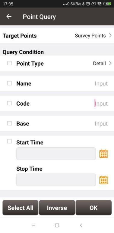
Figure 2.45[]{#_Toc10359 .anchor} Point Query interface
Query condition details are as follows:
[Point Type]: Detail, continuous, input point, calculate or base.
[Name]: Point name to be queried.
[Code]: Code number.
[Base]: The name of the base.
[Start/Stop Time]: Start and stop time of the points
Click [OK] to search all the points meeting the query conditions.
- Delete survey point
In the survey point interface, click [Multiselect], select the points to be deleted and click [Delete] to complete the deletion.
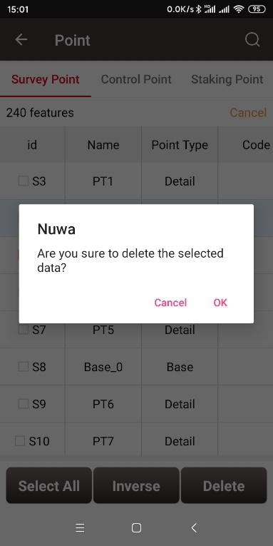 Figure 2.46[]{#_Toc13078 .anchor} Pop-up notice before deletion
Note: The base point in the survey point library cannot be deleted.
2.4.2 Control Point
In Nuwa app, the control points are used in parameter calculation and site calibration.
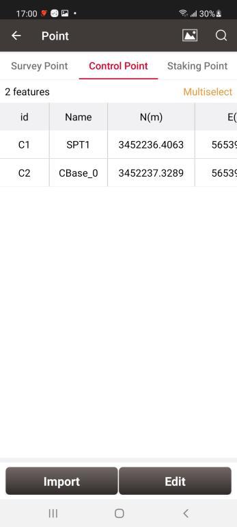
Figure 2.47[]{#_Toc24530 .anchor} Control Point interface
- Import control point
In the Control Point interface, click [Import] to import the control points.
It can be done in three ways: From File, From Survey Point and Manually Add.
Select [From File] to enter the import data interface.
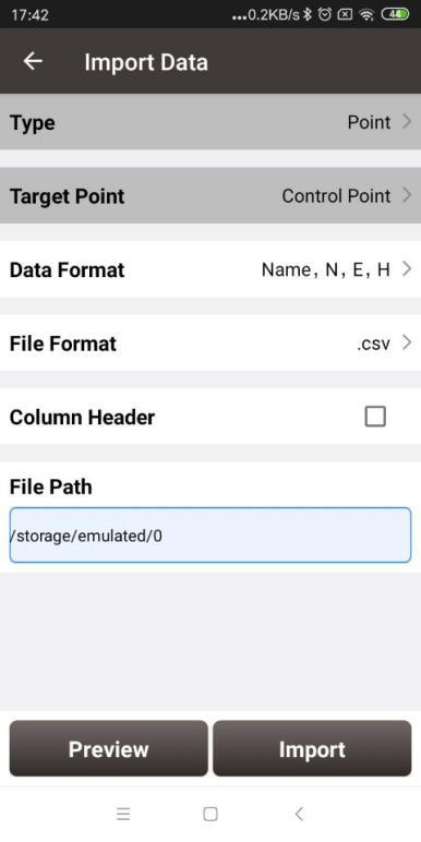
Figure 2.48[]{#_Toc9505 .anchor} Import Data info
Then click [Data format] and select a format in the pop-up list.
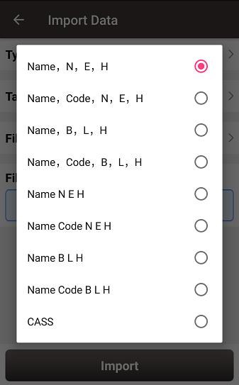
Figure 2.49[]{#_Toc15766 .anchor} Data format list
Select file format and file path to import points. Then click [Import] to import the required points.
Select [From Survey Point] and then select the points in the Survey Point list.
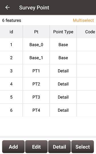
Figure 2.50[]{#_Toc27777 .anchor} Import Survey Point
Select [Manually Add] to enter the Add Control Point interface.
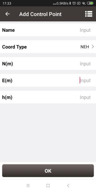
Figure 2.51[]{#_Toc1107 .anchor} Add Control Point
Choose the coordinate type (including two types: BLH and NEH), fill in the point name and the coordinate values, or click the upper right ![]() icon to import the survey point directly.
icon to import the survey point directly.
- Edit control point
In the control point interface, select a control point, click [Edit] to edit control point.
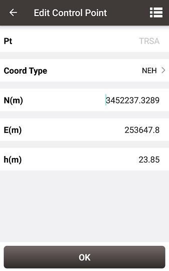
Figure 2.52[]{#_Toc9576 .anchor} Edit Control Point interface
- Query control point
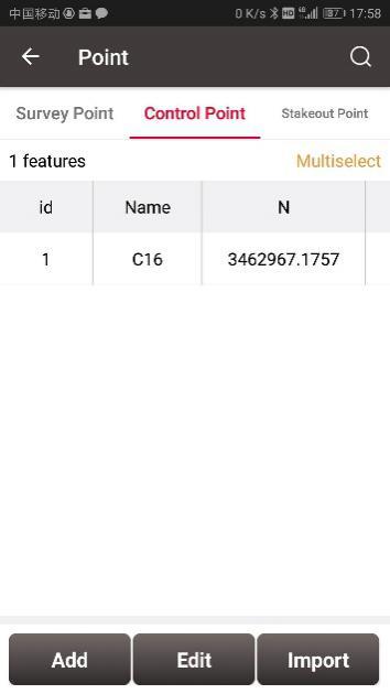
Figure 2.53[]{#_Toc8169 .anchor} Control Point interface
Click the up-right
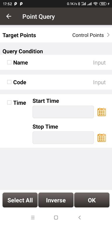
Figure 2.54[]{#_Toc31194 .anchor} Point Query interface
- Delete control point
Click [Multiselect] in the control point interface to enter the following interface. Select the points to be deleted and click [Delete] to complete the deletion.
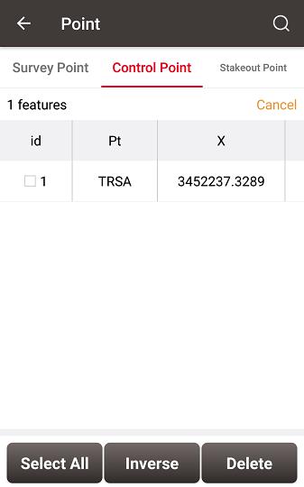
Figure 2.55[]{#_Toc25244 .anchor} Delete Control Point
2.4.3 Staking Point
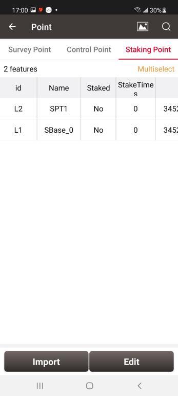
Figure 2.56[]{#_Toc26465 .anchor} Staking Point interface
- Import staking point
In the staking point interface, click [Import] to import staking points.
It can be done in four ways: From Files, From Survey Point, From Control Point, Manually Add.
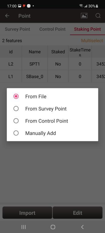
Figure 2.57[]{#_Toc6250 .anchor} Import source for Staking Point
Choosing [From File] leads to the similar steps of importing Control Point.
Choosing [From Survey Point] leads to the figure below. One or more points can be selected and imported as Staking Points.
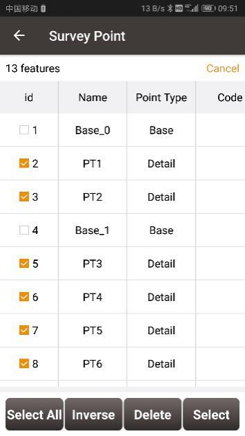
Figure 2.58[]{#_Toc3331 .anchor} Import from Survey Point
Choosing [From Control Point] leads to the control point list. One or more points can be selected and imported as Staking Points.
Choosing [Manually Add] leads to the Add Staking Point interface.
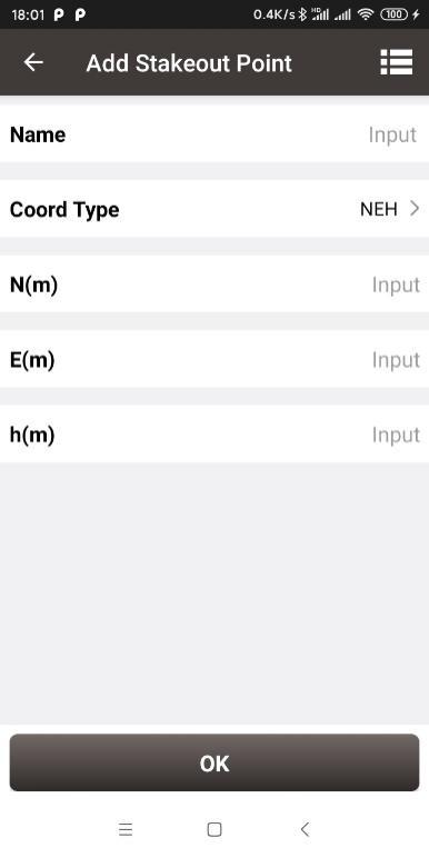
Figure 2.59[]{#_Toc25755 .anchor} Control Point interface
- Edit staking point
In the staking point interface, select a staking point and click [Edit] to enter the editing interface.
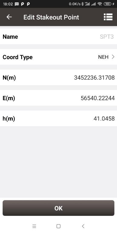 Figure 2.60[]{#_Toc5489 .anchor} Edit Staking Point
- Query staking point
Click the up-right
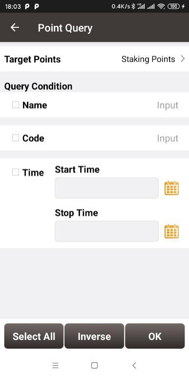 Figure 2.61[]{#_Toc7579 .anchor} Query Staking Point
- Delete staking point
Click [Multiselect] in the staking point interface, select the points to be deleted and click [Delete] to complete the deletion.
2.4.4 DB List
It is supported for a project to contain one or more point library database files. All point library databases under the project use the same coordinate system parameters of the project for the coordinate conversion. And the data between point library DB are independent of each other. Click ![]() on the top right to enter the DB list management interface to create a new point library database and select the point library database.
on the top right to enter the DB list management interface to create a new point library database and select the point library database.
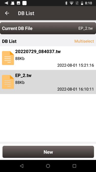
Figure 2.62[]{#_Toc4481 .anchor} Point Database List interface
- Add point database
Click [New], enter the name of the new point database file and click OK, the new point database will be created and opened automatically.
- Open point database
Click on one of the point database and click OK in the prompt dialog to switch to the point database selected.
- Delete point database
Click [Multiselect] in the DB List interface, select the database to be deleted and click [Delete] to complete deletion. The point database opened currently cannot be deleted. After the database file is deleted, all the points in the database will be deleted, so please delete it carefully.
Line
This section includes survey line and staking line.
2.5.1 Survey Line
- Add survey line
Click [Project] - > [Line] and see the Survey Line as below.
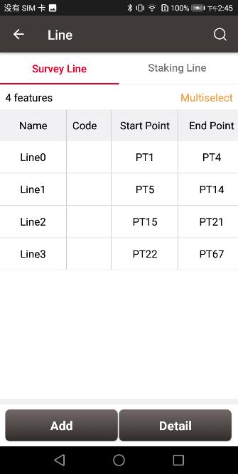
Figure 2.63[]{#_Toc6917 .anchor} Line interface
Click [Add] under Survey Line to enter the following interface.
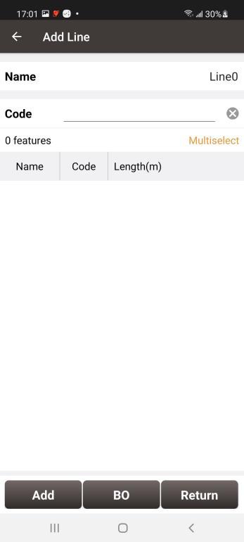
Figure 2.64[]{#_Toc22238 .anchor} Add Survey Line interface
Fill in a line name or use the default name, input a code for comment purpose, click [Add] in the bottom left to select two points in the survey point library as below.
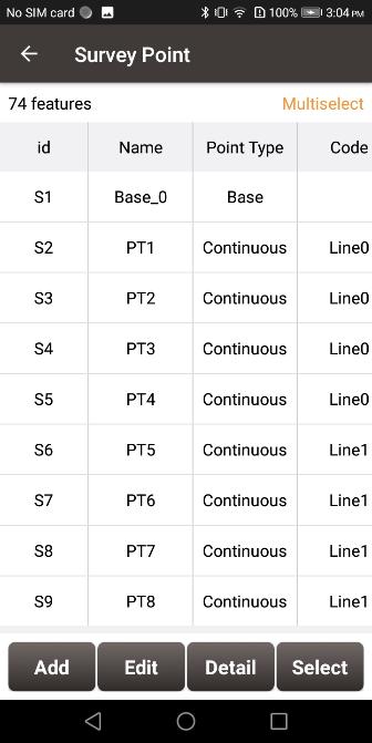
Figure 2.65[]{#_Toc10752 .anchor} Select two points from Survey Point library -- 1
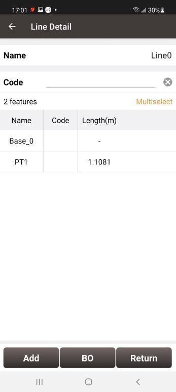
Figure 2.66[]{#_Toc14078 .anchor} Select two points from Survey Point library -- 2
Click [BO] to close the new survey line.
Click [Return] and the new survey line has been added as below.
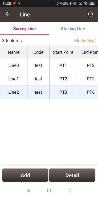
Figure 2.67[]{#_Toc7118 .anchor} Survey Line added
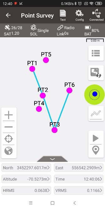
The added survey line can be viewed under [Survey] -> [Point Survey] shown as below.
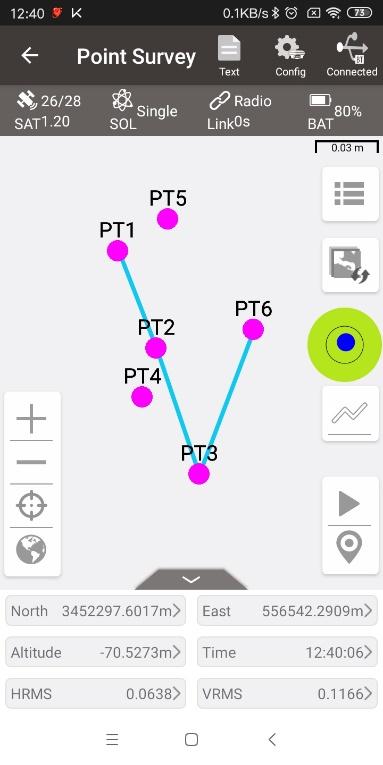
Figure 2.68[]{#_Toc8789 .anchor} Survey Line in Survey interface
- View and edit survey line
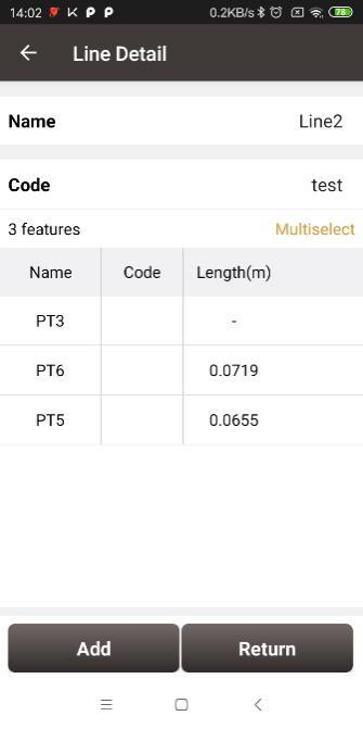
In the Line interface, select the line to be edited. Then click [Detail] to enter the edit page shown as below.
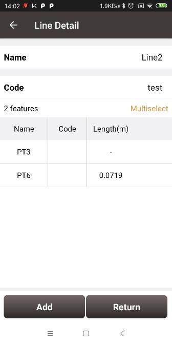
Figure 2.69[]{#_Toc8866 .anchor} Edit the Survey Line Line2
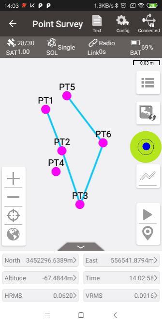
If not selecting a point, click [Add] to add a point at the end shown as Figure 2.69; if selecting a point, then click [Add] to insert a point before the selected point shown as Figure 2.71. After adding the point, the length will be recalculated, and then enter the survey interface to find that the added point is connected to the line shown as Figure 2.70 and Figure 2.72.
+----------------------------------------------------------------------------------------------------------------------------------------------+----------------------------------------------------------------------------------------------------------------------------------------------+
|  |
|  |
| | |
| Figure 2.70[]{#_Toc3017 .anchor} Add PT5 to the line end | Figure 2.71[]{#_Toc28850 .anchor} The new Line2 in survey interface |
+----------------------------------------------------------------------------------------------------------------------------------------------+----------------------------------------------------------------------------------------------------------------------------------------------+
|
|
| | |
| Figure 2.70[]{#_Toc3017 .anchor} Add PT5 to the line end | Figure 2.71[]{#_Toc28850 .anchor} The new Line2 in survey interface |
+----------------------------------------------------------------------------------------------------------------------------------------------+----------------------------------------------------------------------------------------------------------------------------------------------+
|  |
|  |
| | |
| Figure 2.72[]{#_Toc8293 .anchor} Add PT5 before PT6 | Figure 2.73[]{#_Toc19854 .anchor} The new Line2 in survey interface |
+----------------------------------------------------------------------------------------------------------------------------------------------+----------------------------------------------------------------------------------------------------------------------------------------------+
|
| | |
| Figure 2.72[]{#_Toc8293 .anchor} Add PT5 before PT6 | Figure 2.73[]{#_Toc19854 .anchor} The new Line2 in survey interface |
+----------------------------------------------------------------------------------------------------------------------------------------------+----------------------------------------------------------------------------------------------------------------------------------------------+
Click [BO] to close the survey line.
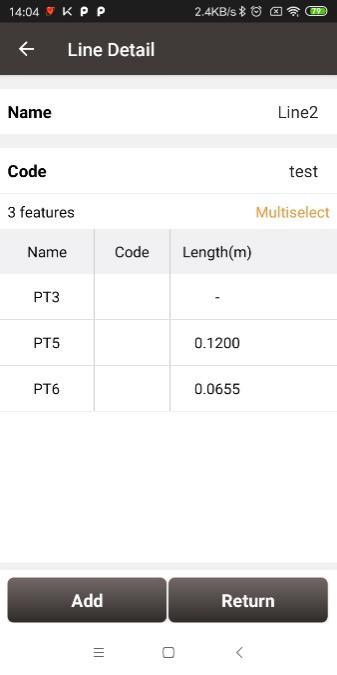
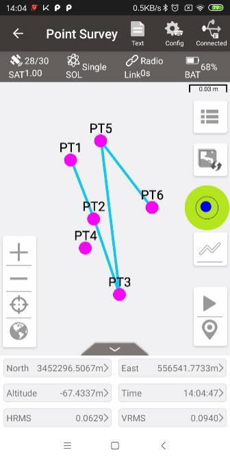
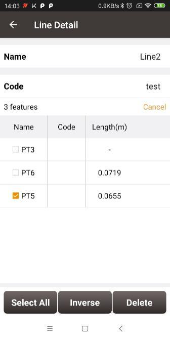
Click [Multiselect] to select a point and click [Delete]. After the deletion, the length will be recalculated, and then enter the survey interface to find that the deleted point is no longer connected to the line. For example, after deleting PT5 in Line2, this point PT5 is no longer in Line2 shown as below.
Note: After deleting the point in the line, the point and its information will be retained in the point library. It exists as a point, but it is no longer connected to the line.
+----------------------------------------------------------------------------------------------------------------------------------------------+----------------------------------------------------------------------------------------------------------------------------------------------+
|  |
|  |
| | |
| Figure 2.74[]{#_Toc10065 .anchor} Delete PT5 in Line2 | Figure 2.75[]{#_Toc5552 .anchor} Line2 after deleting PT5 |
+----------------------------------------------------------------------------------------------------------------------------------------------+----------------------------------------------------------------------------------------------------------------------------------------------+
|
| | |
| Figure 2.74[]{#_Toc10065 .anchor} Delete PT5 in Line2 | Figure 2.75[]{#_Toc5552 .anchor} Line2 after deleting PT5 |
+----------------------------------------------------------------------------------------------------------------------------------------------+----------------------------------------------------------------------------------------------------------------------------------------------+
- Query survey line
Click the ![]() icon at the up-right corner, the line query interface is shown as below. Input the search items and tick the item, click [OK] to search the line.
icon at the up-right corner, the line query interface is shown as below. Input the search items and tick the item, click [OK] to search the line.
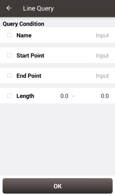
Figure 2.76[]{#_Toc7682 .anchor} Line Query interface
- Delete survey line
In the Survey Line interface, click [Multiselect] to enter the following interface. Tick the line to be deleted, then click [Delete] to complete deletion.
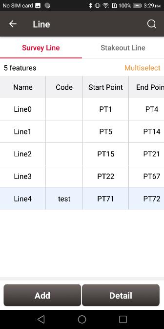
Figure 2.77[]{#_Toc22612 .anchor} Survey line interface
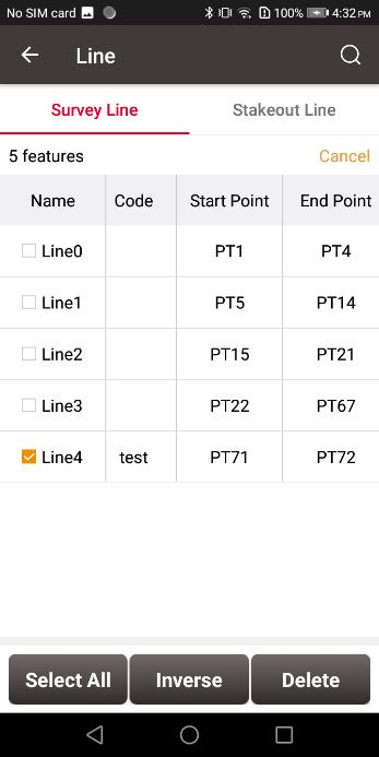
Figure 2.78[]{#_Toc25774 .anchor} Tick the line to be deleted
2.5.2 Staking Line
- Add staking line
Click [Add] under Stakeout Line to enter the following interface, there are four types of staking line: line, polyline, arc and circle.
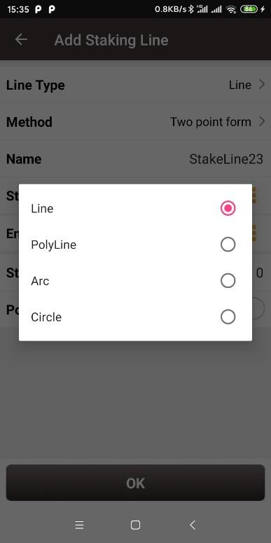
Figure 2.79[]{#_Toc1930 .anchor} Four types of staking line
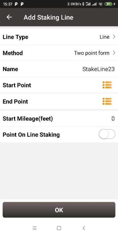
a. Line
+----------------------------------------------------------------------------------------------------------------------------------------------+----------------------------------------------------------------------------------------------------------------------------------------------+
|  |
|  |
| | |
| Figure 2.80[]{#_Toc3843 .anchor} Add line method 1 | Figure 2.81[]{#_Toc28297 .anchor} Add line method 2 |
+----------------------------------------------------------------------------------------------------------------------------------------------+----------------------------------------------------------------------------------------------------------------------------------------------+
|
| | |
| Figure 2.80[]{#_Toc3843 .anchor} Add line method 1 | Figure 2.81[]{#_Toc28297 .anchor} Add line method 2 |
+----------------------------------------------------------------------------------------------------------------------------------------------+----------------------------------------------------------------------------------------------------------------------------------------------+
- Two Points:
Input the name of the line, then click ![]() to import the start point and end point.
to import the start point and end point.
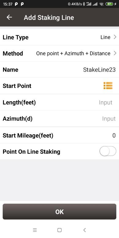
- One point + Azimuth + Distance
Input the name of the line, then click ![]() to import the start point from a point library.
to import the start point from a point library.
Input the other information for the line.
Start Mileage: default is 0. The mileage of other points on the line will be obtained by adding the start mileage and the mileage from the starting point.
Point On Line Staking
-
Turn on this function, you can set the pile interval and the stakeout will start from the starting point of the staking line to the end point at this interval.
-
Turn off this function, the stakeout will be to the vertical cross point between the current position and the staking line (or the extension line).
b. Polyline
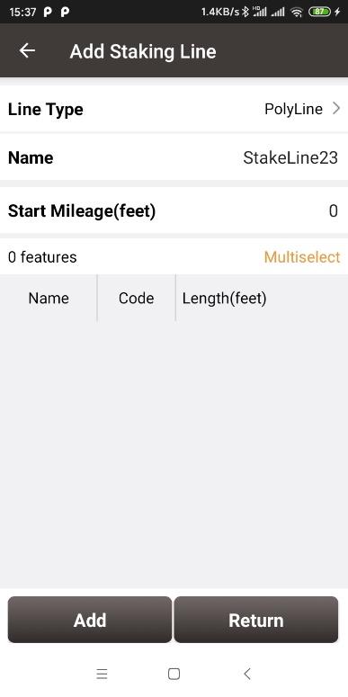
Figure 2.82[]{#_Toc27471 .anchor} Add polyline
Add the points that form the polyline one by one, and click Return to save the polyline as the staking line.
Start Mileage: default is 0. The mileage of other points on the line will be obtained by adding the start mileage and the mileage from the starting point.
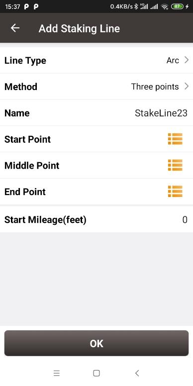
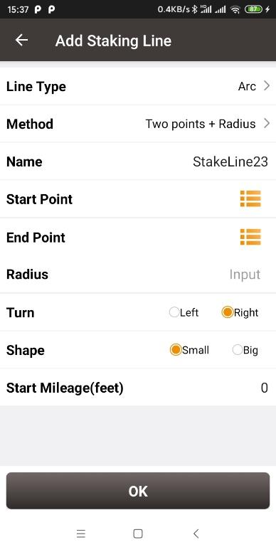
c. Arc
+----------------------------------------------------------------------------------------------------------------------------------------------+----------------------------------------------------------------------------------------------------------------------------------------------+
|  |
|  |
| | |
| Figure 2.83[]{#_Toc7936 .anchor} Add arc method 1 | Figure 2.84[]{#_Toc24115 .anchor} Add arc method 2 |
+----------------------------------------------------------------------------------------------------------------------------------------------+----------------------------------------------------------------------------------------------------------------------------------------------+
|
| | |
| Figure 2.83[]{#_Toc7936 .anchor} Add arc method 1 | Figure 2.84[]{#_Toc24115 .anchor} Add arc method 2 |
+----------------------------------------------------------------------------------------------------------------------------------------------+----------------------------------------------------------------------------------------------------------------------------------------------+
-
Three points: Select the starting point, the middle point and the end point to form the arc.
-
Two points + Radius: Select the starting point and end point, enter the radius, select the turning direction and shape of the arc from the starting point to the end point, the software can automatically calculate the center coordinates of the circle to form the arc.
Start Mileage: default is 0. The mileage of other points on the line will be obtained by adding the start mileage and the mileage from the starting point.
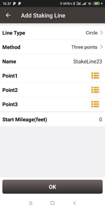
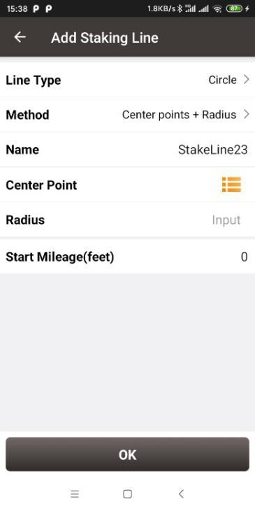
d. Circle
+---------------------------------------------------------------------------------------------------------------------------------------------+---------------------------------------------------------------------------------------------------------------------------------------------+
|  |
|  |
| | |
| Figure 2.85[]{#_Toc25407 .anchor} Add circle method 1 | Figure 2.86[]{#_Toc8573 .anchor} Add circle method 2 |
+---------------------------------------------------------------------------------------------------------------------------------------------+---------------------------------------------------------------------------------------------------------------------------------------------+
|
| | |
| Figure 2.85[]{#_Toc25407 .anchor} Add circle method 1 | Figure 2.86[]{#_Toc8573 .anchor} Add circle method 2 |
+---------------------------------------------------------------------------------------------------------------------------------------------+---------------------------------------------------------------------------------------------------------------------------------------------+
-
Three points: Select three points on the circle to form a circle.
-
Center point + Radius: Select the center of the circle and enter the radius to form the circle.
Start Mileage: default is 0. The mileage of other points on the line will be obtained by adding the start mileage and the mileage from the starting point.
- View and edit staking line
In staking line interface, select a staking line, click [Detail] to enter the edit page and edit the line parameters shown as below.
- Query staking line
Query of a staking line is the same with query of a survey line, enter the line query interface, input the search items and tick the item, click [OK] to search the staking line.
- Delete staking line
Deleting a staking line is the same with deleting a survey line, in the staking line interface, click [Multiselect] and tick the staking line to be deleted, click [OK] to complete the deletion.
Road
Road management is used to create or edit road data.
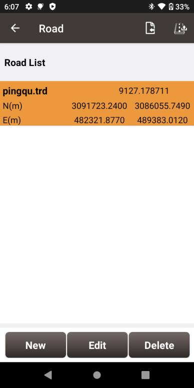
Figure 2.87[]{#_Toc24423 .anchor} Road List interface
2.6.1 Add new road
The road contains a variety of feature factors. The current software supports the use of station equation, intersection method or element method to edit the road's alignment, vertical profile, cross section, super elevation, and widening. Click [Road] -> [New] to enter the Add Road interface. Enter the road name, start miles and parameters of the road.
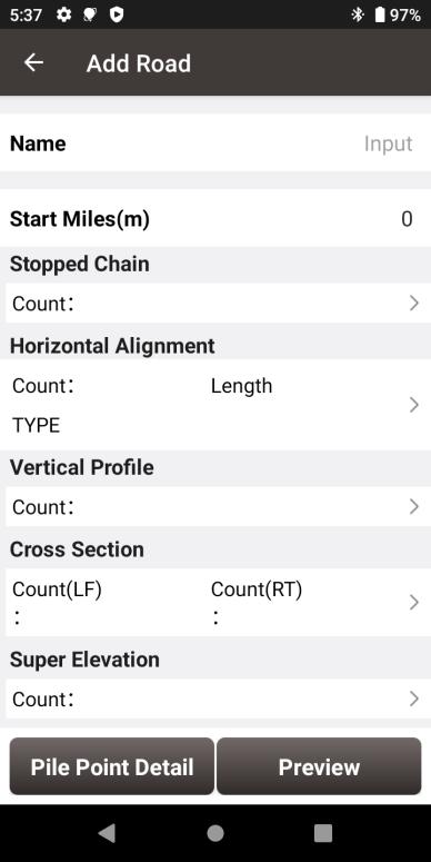
Figure 2.88[]{#_Toc13010 .anchor} Add Road interface
Station equation
A station equation refers to the phenomenon that the stake number is not continued due to stationing changes or section measurement.
Alignment
The horizontal alignment is a curve that describes the turning and trend of the road curve in the horizontal plane. It generally consists of straight lines, arcs, and transition curves. The transition curve used in the calculation of the software is the clothoid (also known as Cornu spiral or Euler spiral) commonly used in road design.
+-----------------------------------------------------------------------------------------------------------------------------------------------------------------------+-----------------------------------------------------------------------------------------------------------------------------------------------------------------------+
|  |
|  |
| | |
| Figure 2.89[]{#_Toc30691 .anchor} Intersection method interface | Figure 2.90[]{#_Toc24744 .anchor} Element method interface |
+-----------------------------------------------------------------------------------------------------------------------------------------------------------------------+-----------------------------------------------------------------------------------------------------------------------------------------------------------------------+
|
| | |
| Figure 2.89[]{#_Toc30691 .anchor} Intersection method interface | Figure 2.90[]{#_Toc24744 .anchor} Element method interface |
+-----------------------------------------------------------------------------------------------------------------------------------------------------------------------+-----------------------------------------------------------------------------------------------------------------------------------------------------------------------+
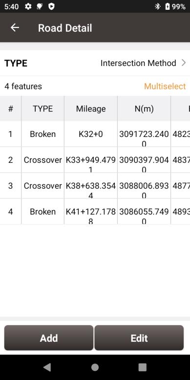
Alignment - Intersection method
The intersection method is based on the intersection point in the alignment, and the coordinates are obtained through the intersection point and the route. The general intersection point method to construct an alignment consists of a starting polyline point, N intersection points and an ending polyline point. Enter the coordinates of the designed road at the starting and ending polyline points; the intersection needs to enter the coordinates of the designed intersection point, the length of the entry transition curve, the radius and the length of the exit transition curve. The software will automatically calculate the elements contained under the intersection and draw the road alignment.
The current software supports the conversion calculation from the intersection method to the element method; supports the input of the intersection method of the complete symmetric transition curve and the complete asymmetric transition curve; supports the intersection method input when the transition curve length is 0 or the arc length is 0; it does not support the input of incomplete transition curve; it does not support the intersection method input of special curve such as a turning curve.
Alignment - Element method
The element method is a method to calculate the alignment coordinates from the node elements such as the starting point coordinates, azimuth angle, starting point stake number and ending point stake number of the road. Select the corresponding elements when entering the element method, including straight lines, left-turning arcs, right-turning arcs, left-turning transition curves, right-turning transition curves, and then input the corresponding feature parameters of the elements, such as the length, start radius and end radius of the transition curve. The software will draw a road alignment according to the input line elements.
Vertical Profile
A vertical profile refers to the curve that connects two adjacent wavebands on the vertical section of the line with the slope point as the intersection point. The vertical profile describes the change of the elevation coordinate of the middle stake point. The vertical profile in the software is calculated using a parabola.
Cross Section
The cross section refers to the section perpendicular to the center line of the road at the center pile. The main components include motor vehicle lanes, non-motor vehicle lanes, sidewalks, hard shoulders, soil shoulders, central separation belts, and side partitions.
The cross section need to be established on the vertical profile.
The super-elevation and widening properties in the software need to be established on the basis of the standard cross section.
Super Elevation
When a vehicle is driving on a curve, it will slip due to lateral force or centrifugal force. In order to offset the centrifugal force generated by the vehicle driving on the curve and ensure that the vehicle passes the curve safely and stably, a unidirectional cross-slope that is higher on the outside than the inside will be set on the cross section of the curved road section, which is the super-elevation property of the road. The superelevation of the road in the software is based on the standard cross-section, which will be reflected in the changes in the slope of the plates composed of different cross-sections, and will ultimately affect the change of the elevation coordinates of the side piles.
Widening
When the vehicle is driving on a curve, the driving trajectory of each wheel is different. The radius of the driving trajectory of the rear wheel on the inner side of the curve is the smallest, and the radius of the driving trajectory of the front wheel near the outer side of the curve is the largest. This phenomenon is more prominent when the radius of the driving curve is small. In order to ensure that the car does not encroach on the adjacent lanes when turning, the curved road sections need to be widened. The widening of the road in the software will be based on the standard cross-section, which will be reflected in the changes in the width of the plates composed of different cross-sections, and will ultimately affect the change of the side pile coordinates.
After the road parameters input is completed, use [Pile Point Detail] and [Preview] to check and confirm the road data.
Pile Point Detail
Click [Pile Point Detail] to enter the interface, input the start mileage and set the interval to check the road, then set the storage path. Click [Query] to show the coordinates of the point on the road in list, and click [Export] to export the road data list to the designated folder.
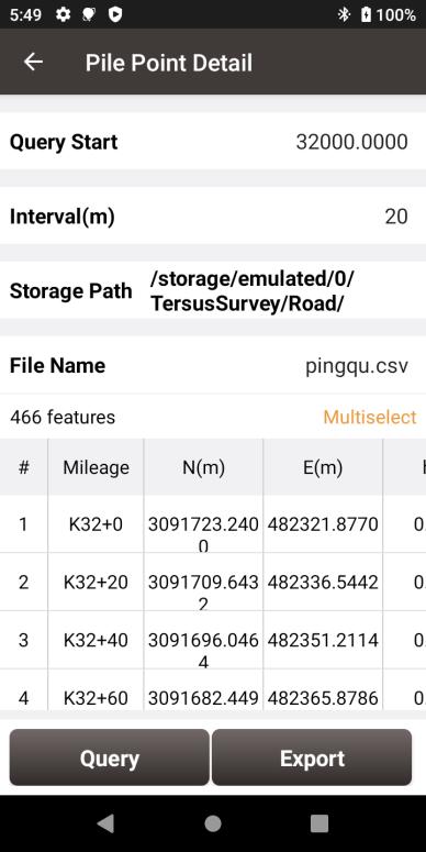
Figure 2.91[]{#_Toc27262 .anchor} Pile Point Detail
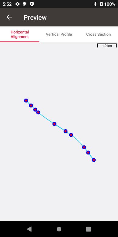
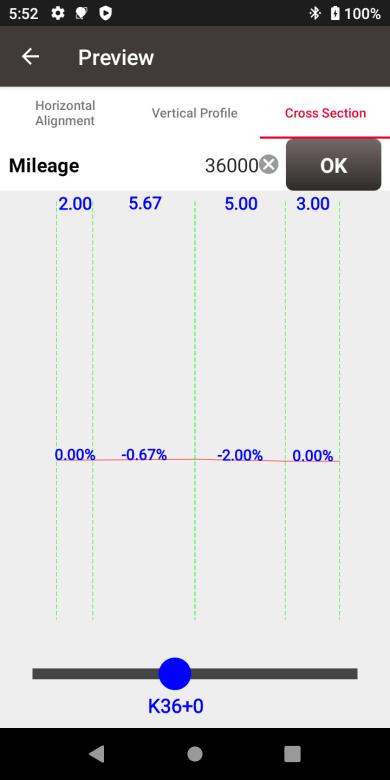
Preview
Click [Preview] to enter the interface, click [Horizontal Alignment] to show the graphics of the road route in the overhead direction, to judge whether the alignment parameters input are abnormal by the road shape; click [Vertical Profile] to show the elevation change along the center-line of the road, and enter the mileage or drag the red line to query the elevation of specified mileage; click [Cross Section] to show the road cross-section changes, and enter the mileage or drag the bottom progress bar to display the cross section at the specified mileage.
+------------------------------------------------------------------------------------------------------------------------------------------------------------+----------------------------------------------------------------------------------------------------------------------------------------------------------------------+
|  |
|  |
| | |
| Figure 2.92[]{#_Toc12204 .anchor} Preview Alignment | Figure 2.93[]{#_Toc32478 .anchor} Preview Cross Section |
+------------------------------------------------------------------------------------------------------------------------------------------------------------+----------------------------------------------------------------------------------------------------------------------------------------------------------------------+
|
| | |
| Figure 2.92[]{#_Toc12204 .anchor} Preview Alignment | Figure 2.93[]{#_Toc32478 .anchor} Preview Cross Section |
+------------------------------------------------------------------------------------------------------------------------------------------------------------+----------------------------------------------------------------------------------------------------------------------------------------------------------------------+
2.6.2 Edit road
In the road interface, choose a road file and click [Edit] to make edition of the existing road.
If the road alignment is created by the intersection method, then it is to edit using the intersection method by default; if the road alignment is created by the element method, then it is to edit using the element method by default. If the road is created by the intersection method, after using the software to switch to the element method, click [Edit], then the software will pop up a prompt asking whether to change from the intersection method to the element method. This mode modification is irreversible.
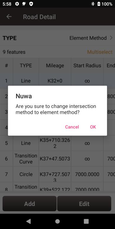
Figure 2.94[]{#_Toc12128 .anchor} Change method when editing road
2.6.3 Delete road
Choose a road file in the road interface, click [Delete] to delete this existing road.
2.6.4 Import/Export road
Tersus road files are in .trd format and stored in the TersusSurvey\Road folder. If a road is created on the Nuwa software of another controller, you can copy the .trd file to this path and open the Nuwa software to load the road.
In the Road interface, click the icon ![]() , select the road file in LandXML or PHI format, and click [Import] to import the alignment, vertical profile and cross section data.
, select the road file in LandXML or PHI format, and click [Import] to import the alignment, vertical profile and cross section data.
In the Road interface, select the road, click the icon  , set the storage path to export the cross-section survey data to the designated folder.
Import
There are two types of import: Coordinate Import and Other Import. Coordinate import is to import files with .csv and .dat format. Other Import is to import files with .dxf, .shp and .sima format.
2.7.1 Coordinate Import
Under the Coordinate Import interface, select Type, Target Point library to be added, Data Format, File Format and the file path where the file is located, click [Import] to complete the import.
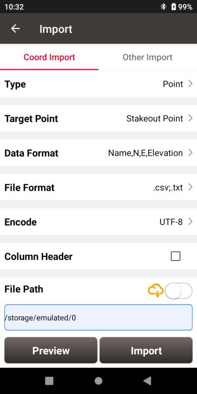
Figure 2.95[]{#_Toc8269 .anchor} Import interface
The figure above shows the parameters that should be selected or filled for coordinate import.
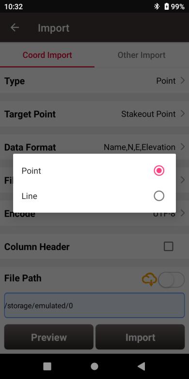
Figure 2.96[]{#_Toc521 .anchor} Import Type
For point import, select [Point] for Type as shown above.
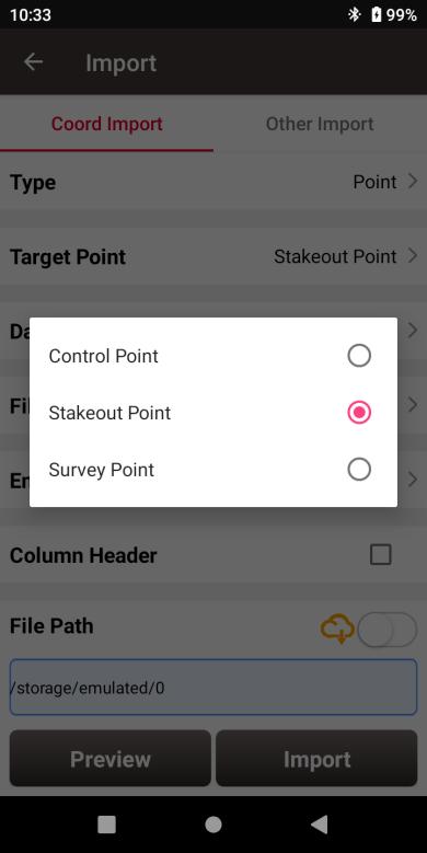
Figure 2.97[]{#_Toc17600 .anchor} Target Point Library
The target point library has three options: control point, stakeout point and survey point as shown above.
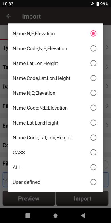
Figure 2.98[]{#_Toc7112 .anchor} Data Format options
The data format options for data import are listed in the figure above.
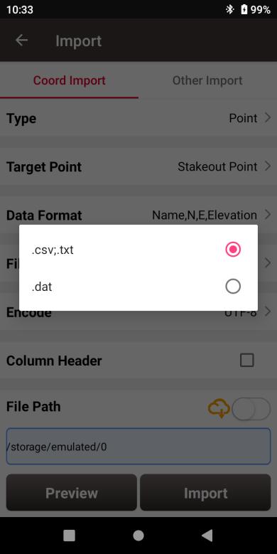
Figure 2.99[]{#_Toc17681 .anchor} File Format options
There are two options for file format of imported points: .csv;.txt and .dat files.
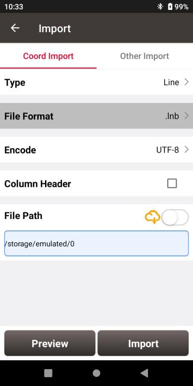
Figure 2.100[]{#_Toc32007 .anchor} Import Line interface
For line import, select [Line] for Type in Figure 2.94 and it goes to the import line interface as shown in Figure 2.98 above. The file format for line is .lnb file.
The line file is a text file with the .lnb extension in nature. The detailed content in the text file is shown as below. The information from left to right is: starting point name, starting point N, starting point E, starting point h, 0, ending point name, ending point N, ending point E, ending point h, 0, 0.

Figure 2.101[]{#_Toc2704 .anchor} Example content in the .lnb file
2.7.2 Other Import
Under the Other Import interface, select the file format, type, target point and the file path, click [Import] to import the file. Now Nuwa supports importing DXF, SHP, SIMA, KML, KMZ, NCN and LandXML files. And the Type can be selected as vector base map when the file format is DXF, SHP, KML/KMZ, LandXML and other supported formats. The imported vector map can be selected and displayed in the Survey and Stakeout interface after import. When the Type is selected as point, the target point library can be selected as Survey Point, Control Point and Staking Point.
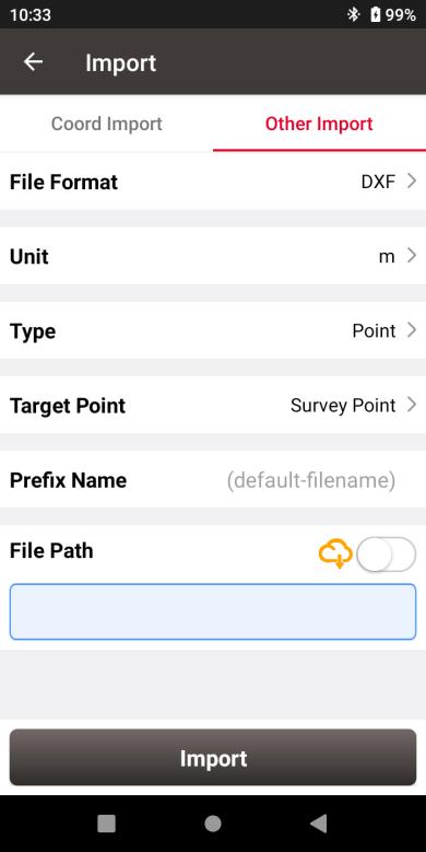
Figure 2.102[]{#_Toc27670 .anchor} Other Import interface
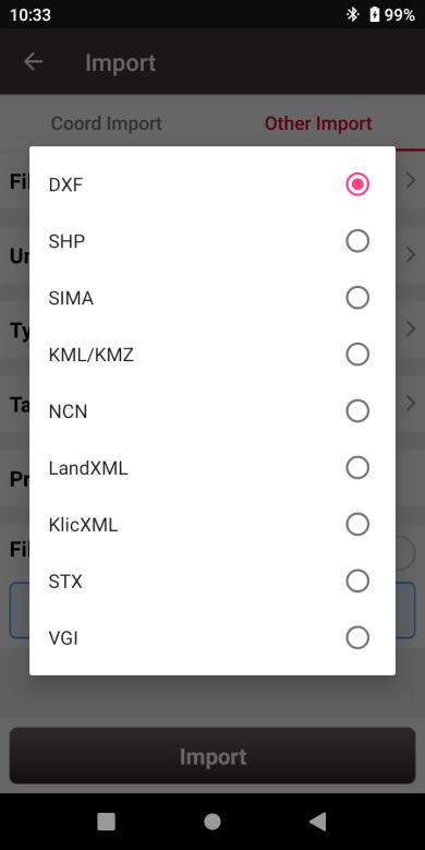
Figure 2.103[]{#_Toc13754 .anchor} File format for other import
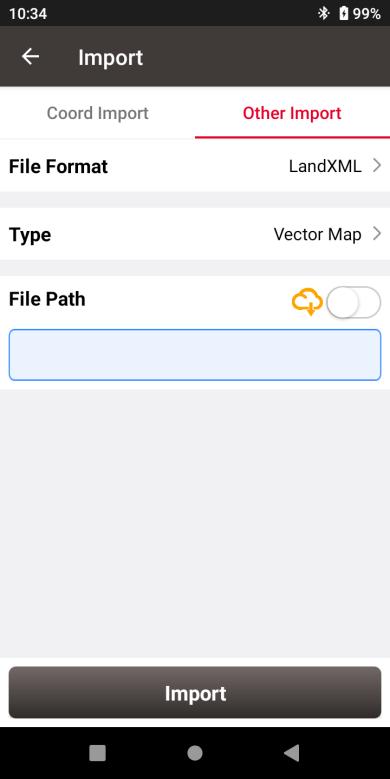
Figure 2.104[]{#_Toc29206 .anchor} Import as Vector Map
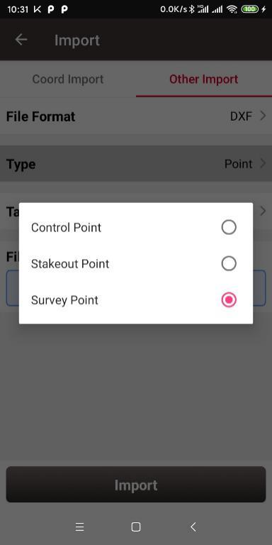
Figure 2.105[]{#_Toc8776 .anchor} Target point options
Export
Correspondingly there are two types of export: Coordinate Export and Other Export. Coordinate Export is to export .csv files whose file name extension can be modified as .dat; Other Export is to export files with KML, DXF, SHP, HTML, LandXML, and other supported formats.
2.8.1 Coordinate Export
Under the Coordinate Export interface, select Point Type, Date range and Data Format, ensure the File Name and Storage Path is correct.
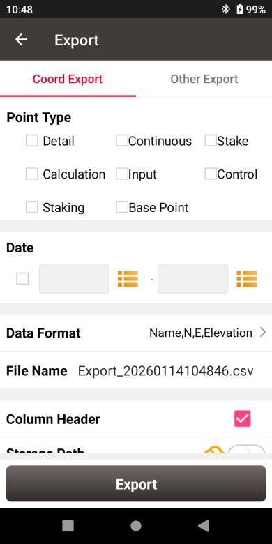
Figure 2.106[]{#_Toc7959 .anchor} Export Interface
Thereafter click [Export] to complete the export.
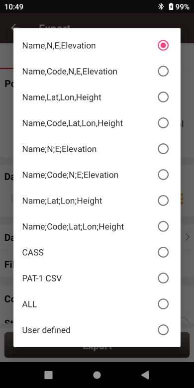
Figure 2.107[]{#_Toc29131 .anchor} Data Format options
For Data Format, the user-defined format can be created or managed. Click [User defined] and it prompts out an option for data format: create data format and manage data format which are shown as below.
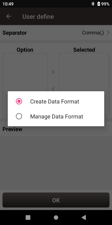
Figure 2.108[]{#_Toc23383 .anchor} User defined data
+----------------------------------------------------------------------------------------------------------------------------------------------------------------------+---------------------------------------------------------------------------------------------------------------------------------------------------------------------+
|  |
|  |
| | |
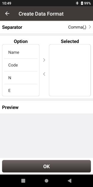
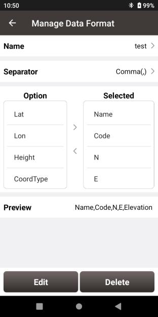
| Figure 2.109[]{#_Toc15528 .anchor} Create data format | Figure 2.110[]{#_Toc21758 .anchor} Manage data format |
+----------------------------------------------------------------------------------------------------------------------------------------------------------------------+---------------------------------------------------------------------------------------------------------------------------------------------------------------------+
|
| | |
| Figure 2.109[]{#_Toc15528 .anchor} Create data format | Figure 2.110[]{#_Toc21758 .anchor} Manage data format |
+----------------------------------------------------------------------------------------------------------------------------------------------------------------------+---------------------------------------------------------------------------------------------------------------------------------------------------------------------+
2.8.2 Other Export
Under the Other Export interface, file format can be KML, SHP, DXF, HTML, LandXML and other supported formats. Type in the export file name and click [Export] to complete the file export.
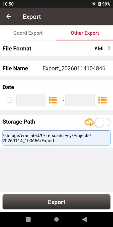
Figure 2.111[]{#_Toc19156 .anchor} Other Export interface
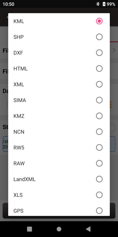
Figure 2.112[]{#_Toc16158 .anchor} File Format for other export
If selecting XML for the file format, select start date and stop date of the Stop&Go survey to ensure the XML file recorded the correct stop points during the Stop&Go survey work.
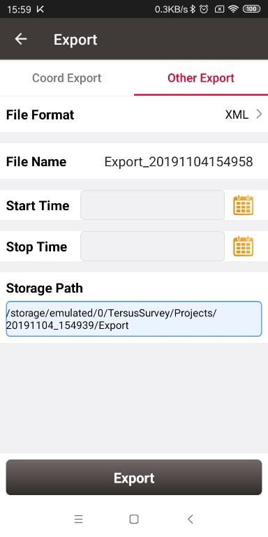
Figure 2.113[]{#_Toc30269 .anchor} Export XML file
Copy the XML file to a computer and open this XML file using a text reader software. Change the rover observation file name on the fifth row to the rover Rinex file name which is shown as below.
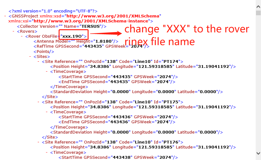
Figure 2.114[]{#_Toc29053 .anchor} Preview of the XML file in text mode
Import the base observation file, rover observation file and the edited XML file to EZSurv application, and EZSurv will identify these files successfully.
Settings
Settings interface is shown as below, the function descriptions is as follows.
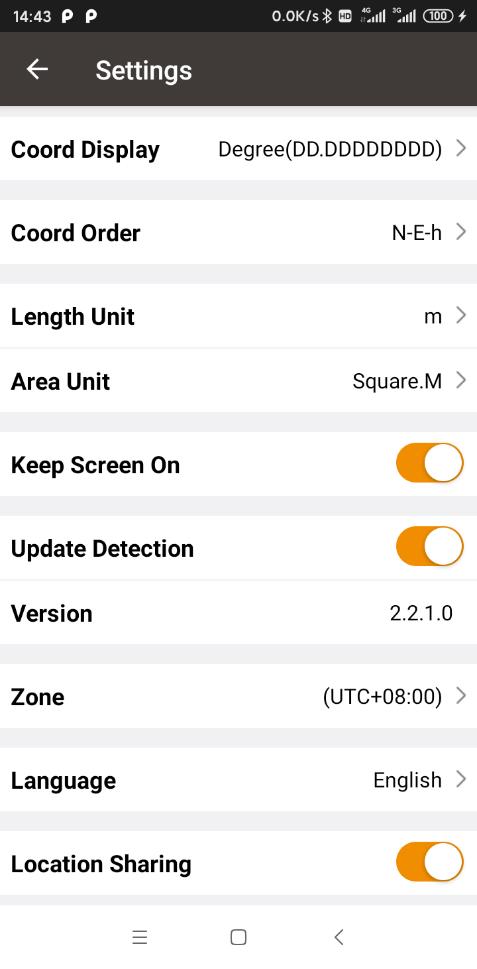
Figure 2.115[]{#_Toc17799 .anchor} Settings interface
[Coord Display]: can be selected from degree (DD.DDDDDDDDD), DM (DD:MM.MMMM) or DMS (DD:MM:SS.SS).
[Coord Order]: the coordinate display order can be NEh, ENh, xyh or yxh. The display order of north and east coordinates will be displayed in the software according to the selected coordinate type format.
[Length Unit]: can be selected from Km, meter, Inch, Feet or US feet.
[Area Unit]: can be selected from Mu, Square Km, Square Meter, Hectare and Acre.
[Distance Decimal]: the number of display and export decimal places for coordinate values and length values can be set.
[Normally On]: the screen would be always on if it is enabled. If on, it is recommended to manually turn off the screen in time to save power when not using the controller.
[Update Detection]: Auto update detection is on if it is enabled.
[Version]: the current version of the Nuwa app.
[Zone]: select the time zone according to the current position.
[Language]: support Auto, Chinese, English, French, Spanish, German, Portuguese, Italian, Russian, Japanese, Korean, Malay, Arabic, Thai, Turkish, Greek, Bulgarian, and Traditional Chinese.
[Location Sharing]: if it is enabled, it will automatically jump to the android system setting interface. Select Nuwa for the mock location app, the location would be shared with other apps.
[Controller Voice]: if it is enabled, after configuring TTS engine and language in the controller system settings - language settings - Text-To-Speech (TTS) output, Nuwa will broadcast the voice when setting the base / rover mode and the solution status change.
When Nuwa app is connected with Oscar GNSS Receiver or Luka GNSS Receiver, you can choose whether to shut down the receiver if you try to exit Nuwa app.
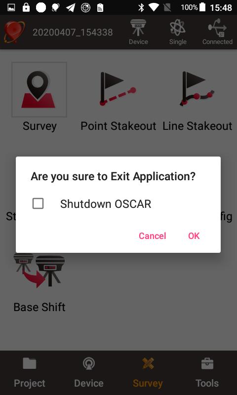
Figure 2.116[]{#_Toc7540 .anchor} Check if shut down Oscar
Cloud Setting
Settings and configuration to use Tersus Cloud.
Tersus GNSS Cloud service is a service that provides users of Tersus software with on cloud data storage, synchronization and management functions. You can register an account through email to use Tersus Cloud, or directly apply for an account from Tersus support team. Enter the server address cloud.tersus-gnss.com, and the correct user name and password, then check to agree to the Legal Notice and Privacy Policy, to log in to Tersus Cloud.
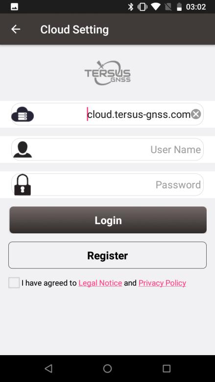
Figure 2.117[]{#_Toc5982 .anchor} Login interface in Cloud Setting
If you do not have an account and need to register, click the [Register] button on the page or log in to the cloud.tersus-gnss.com page on the browser then click the register button. Enter your email address, click [Request verification link], then click the verification link in the email you receive and follow the operation guide to enter your password to complete the creation of your Tersus Cloud account.
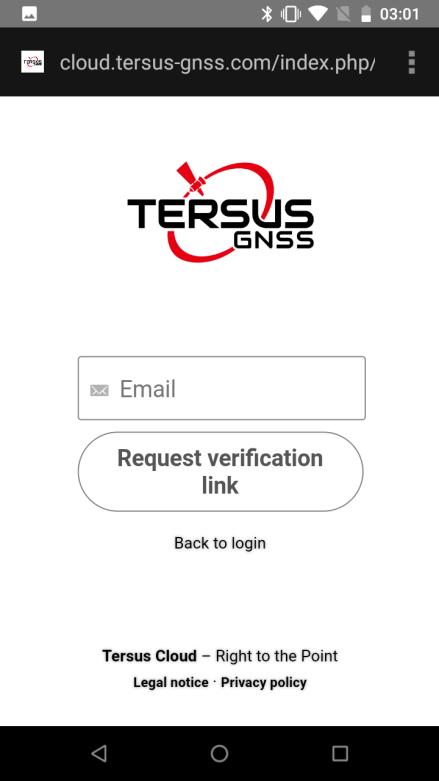
Figure 2.118[]{#_Toc20138 .anchor} Registration interface
After logging in to Tersus Cloud, the interface is as follows. Click [Sync] to synchronize the projects in the controller and on the cloud. After clicking [Sync], the software will automatically judge whether each project need to be uploaded or downloaded according to the update time of project. You can also manually edit the upload or download status of each project, to finish the synchronization.
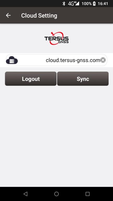
Figure 2.119[]{#_Toc28496 .anchor} Sync projects after login
Tersus Cloud can also be used for uploading and downloading individual projects, importing and exporting data files, coordinate system .csd files, point cloud .las files and more. After logging in to Tersus Cloud, enter the project list screen, click the icon in the upper tight corner to select the current project to upload or download a project from the cloud. Enter the data import screen and choose to import data from the cloud, or enter the data export screen and choose to export data to the cloud.
Log in to Tersus Cloud cloud.tersus-gnss.com through a browser. There, the projects synchronized or uploaded from the controller are stored in /Oscar/Project path. And the data files exported from the controller to the cloud, or the data files for importing from the cloud are stored in /Oscar/Data path. Before importing files from Cloud to Nuwa, please ensure the file exist under the correct path in Tersus Cloud. Please do not place the file in other paths or custom folders, as Nuwa will be unable to locate the file for importing under the specified path.
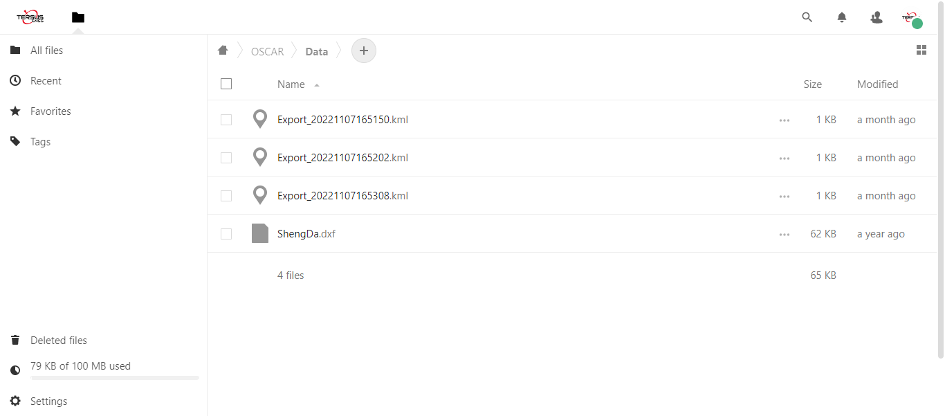
Figure 2.120[]{#_Toc14909 .anchor} Data on Tersus Cloud
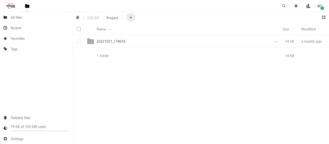
Figure 2.121[]{#_Toc13297 .anchor} Projects on Tersus Cloud